|
|
|
|
35 μm
|
|||
|
25 μm
|
|||
|
105 μm
|
|
1
|
|
2
|
In the Select Physics tree, select Structural Mechanics > Thermal–Structure Interaction > Thermal Stress, Solid.
|
|
3
|
Click Add.
|
|
4
|
Click
|
|
5
|
|
6
|
Click
|
|
1
|
|
2
|
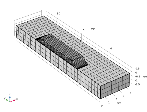
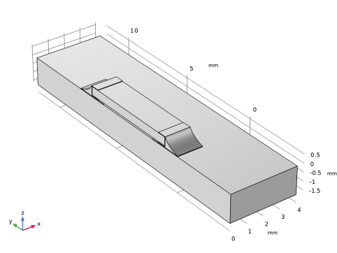
Browse to the model’s Application Libraries folder and double-click the file surface_resistor_geom_sequence.mph.
|
|
3
|
|
1
|
|
2
|
|
1
|
|
2
|
Go to the Add Material window.
|
|
3
|
|
4
|
Click the Add to Component button in the window toolbar.
|
|
5
|
|
6
|
Click the Add to Component button in the window toolbar.
|
|
7
|
|
8
|
Click the Add to Component button in the window toolbar.
|
|
9
|
In the tree, select Material Library > Elements > Silver > Silver [solid] > Silver [solid,annealed].
|
|
10
|
Click the Add to Component button in the window toolbar.
|
|
11
|
|
12
|
Click the Add to Component button in the window toolbar.
|
|
13
|
|
14
|
Click the Add to Component button in the window toolbar.
|
|
15
|
|
1
|
|
2
|
|
3
|
Click
|
|
1
|
|
1
|
|
1
|
|
1
|
|
1
|
|
1
|
|
2
|
|
3
|
|
4
|
|
5
|
|
1
|
|
1
|
|
2
|
|
3
|
|
1
|
|
1
|
|
3
|
|
4
|
From the list, choose Free displacement.
|
|
1
|
|
3
|
|
4
|
From the list, choose Free displacement.
|
|
1
|
|
3
|
|
4
|
|
1
|
|
1
|
|
3
|
|
4
|
|
5
|
|
1
|
|
3
|
|
4
|
|
5
|
|
6
|
|
1
|
|
2
|
|
3
|
|
1
|
|
1
|
|
3
|
|
4
|
Click the Custom button.
|
|
5
|
Locate the Element Size Parameters section.
|
|
6
|
|
1
|
|
1
|
|
2
|
|
3
|
Click the Custom button.
|
|
4
|
Locate the Element Size Parameters section.
|
|
5
|
|
1
|
|
2
|
|
3
|
|
5
|
|
6
|
Locate the Element Size Parameters section.
|
|
7
|
|
1
|
|
2
|
|
3
|
|
4
|
|
1
|
|
2
|
|
3
|
In the Model Builder window, expand the Study 1 > Solver Configurations > Solution 1 (sol1) > Stationary Solver 1 node, then click Segregated 1.
|
|
4
|
|
5
|
|
6
|
In the Model Builder window, expand the Study 1 > Solver Configurations > Solution 1 (sol1) > Stationary Solver 1 > Segregated 1 node, then click Temperature.
|
|
7
|
|
8
|
|
9
|
|
10
|
In the Model Builder window, under Study 1 > Solver Configurations > Solution 1 (sol1) > Stationary Solver 1 > Segregated 1 click Solid Mechanics.
|
|
11
|
|
12
|
|
13
|
|
14
|
|
1
|
|
2
|
|
3
|
Click
|
|
4
|
|
5
|
Click OK.
|
|
6
|
|
8
|
Click
|
|
9
|
|
10
|
Click OK.
|
|
11
|
|
13
|
Click
|
|
1
|
|
1
|
Go to the Result Templates window.
|
|
2
|
|
3
|
Click the Add Result Template button in the window toolbar.
|
|
4
|
|
1
|
|
2
|
|
1
|
|
2
|
|
3
|
|
4
|
|
1
|
|
2
|
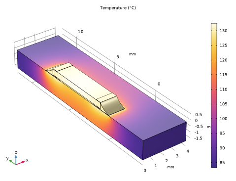
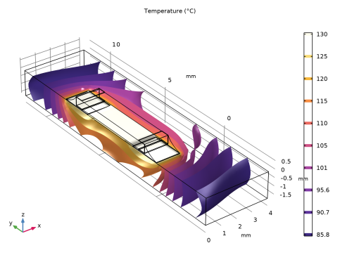
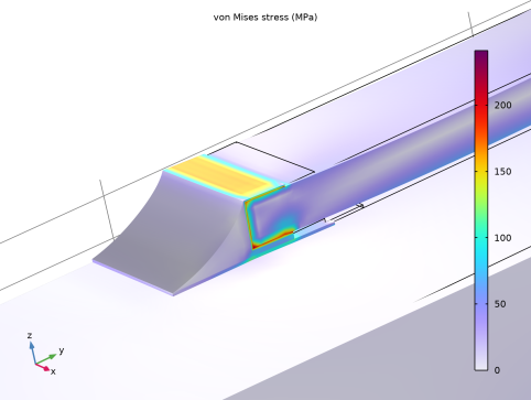
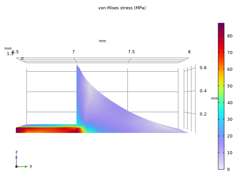
In the Settings window for Volume, click Replace Expression in the upper-right corner of the Expression section. From the menu, choose Component 1 (comp1) > Solid Mechanics > Stress > solid.misesGp - von Mises stress - N/m².
|
|
3
|
|
1
|
|
1
|
|
2
|
|
3
|
|
1
|
|
2
|