|
|
|


|
1
|
|
2
|
|
3
|
Click Add.
|
|
4
|
Click
|
|
5
|
|
6
|
Click
|
|
1
|
|
2
|
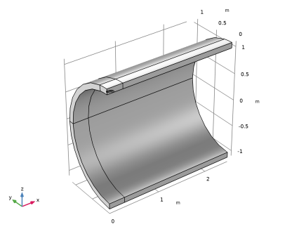
Browse to the model’s Application Libraries folder and double-click the file surface_cracked_cylinder_geom_sequence.mph.
|
|
3
|
|
4
|
|
1
|
|
2
|
|
1
|
|
2
|
|
1
|
|
1
|
|
3
|
|
4
|
|
1
|
|
3
|
|
4
|
|
5
|
|
1
|
|
3
|
|
4
|
|
5
|
|
1
|
|
2
|
|
3
|
|
1
|
|
2
|
|
3
|
Click the Custom button.
|
|
4
|
|
5
|
|
1
|
|
1
|
|
2
|
|
3
|
|
5
|
|
6
|
Locate the Element Size Parameters section.
|
|
7
|
|
8
|
|
9
|
|
10
|
|
1
|
|
2
|
|
3
|
|
5
|
Click to expand the Sweep Method section. From the Destination mesh generation list, choose Morph source onto destination.
|
|
1
|
|
2
|
|
3
|
|
4
|
|
5
|
|
6
|
Select the Reverse direction checkbox.
|
|
7
|
|
1
|
|
2
|
|
3
|
|
5
|
|
1
|
|
2
|
|
3
|
|
1
|
|
2
|
|
3
|
|
4
|
|
5
|
|
6
|
|
1
|
|
2
|
|
3
|
|
4
|
|
5
|
|
1
|
|
2
|
|
3
|
Clear the Plot dataset edges checkbox.
|
|
4
|
|
1
|
|
2
|
Go to the Result Templates window.
|
|
3
|
|
4
|
Click the Add Result Template button in the window toolbar.
|
|
5
|
|
1
|
|
2
|
Go to the Result Templates window.
|
|
3
|
|
4
|
Click the Add Result Template button in the window toolbar.
|
|
5
|
|
1
|
|
2
|
|
3
|
|
5
|
Locate the Variables section. In the table, enter the following settings:
|
|
1
|
|
2
|
|
3
|
|
4
|
|
5
|
|
6
|
|
1
|
|
2
|
|
1
|
|
2
|
|
3
|
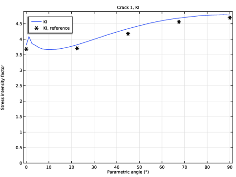
Click Replace Expression in the upper-right corner of the y-Axis Data section. From the menu, choose Component 1 (comp1) > Solid Mechanics > Cracks > solid.crack1.jint1.KI - Stress intensity factor, mode I.
|
|
4
|
|
1
|
|
2
|
|
3
|
Select the x-axis label checkbox.
|
|
4
|
|
5
|
|
6
|
|
7
|
|
1
|
|
2
|
|
3
|
Click
|
|
4
|
Browse to the model’s Application Libraries folder and double-click the file surface_cracked_cylinder_results.txt.
|
|
1
|
|
2
|
|
3
|
|
4
|
|
5
|
|
6
|
|
1
|
|
2
|
|
3
|
Select the Show legends checkbox.
|
|
4
|
|
1
|
|
2
|
|
3
|
Select the Show legends checkbox.
|
|
4
|
|
5
|
Select the Label checkbox.
|
|
1
|
|
2
|
|
3
|
Select the Show legends checkbox.
|
|
4
|
|
1
|
|
2
|
Go to the Result Templates window.
|
|
3
|
In the tree, select Study 1/Solution 1 (sol1) > Solid Mechanics > Fracture Mechanics Results (solid).
|
|
4
|
Click the Add Result Template button in the window toolbar.
|
|
5
|