
|
|
|

|
1
|
|
2
|
|
3
|
Click Add.
|
|
4
|
Click
|
|
5
|
|
6
|
Click
|
|
1
|
|
2
|
|
3
|
|
4
|
|
5
|
Click
|
|
1
|
|
1
|
|
1
|
|
3
|
|
4
|
|
5
|
Specify the M vector as
|
|
6
|
|
7
|
In the Show More Options dialog, in the tree, select the checkbox for the node Physics > Equation Contributions.
|
|
8
|
Click OK.
|
|
1
|
|
3
|
|
4
|
|
1
|
|
2
|
In the Settings window for Auxiliary Dependent Variable, locate the Auxiliary Dependent Variable section.
|
|
3
|
|
4
|
|
5
|
|
1
|
In the Model Builder window, under Component 1 (comp1) right-click Materials and choose Blank Material.
|
|
2
|
|
4
|
|
1
|
|
2
|
Right-click Component 1 (comp1) > Materials > Material 1 (mat1) > Young’s modulus and Poisson’s ratio (Enu) and choose Functions > Piecewise.
|
|
3
|
|
4
|
|
5
|
|
6
|
|
7
|
Find the Intervals subsection. In the table, enter the following settings:
|
|
1
|
In the Model Builder window, under Component 1 (comp1) > Materials > Material 1 (mat1) click Young’s modulus and Poisson’s ratio (Enu).
|
|
2
|
In the Settings window for Young’s Modulus and Poisson’s Ratio, locate the Output Properties section.
|
|
1
|
|
3
|
|
4
|
|
1
|
|
3
|
|
4
|
|
5
|
Click
|
|
1
|
|
2
|
|
3
|
In the Model Builder window, expand the Study 1 > Solver Configurations > Solution 1 (sol1) > Stationary Solver 1 node, then click Fully Coupled 1.
|
|
4
|
|
5
|
|
6
|
|
1
|
|
2
|
|
3
|
|
1
|
|
2
|
Go to the Result Templates window.
|
|
3
|
In the tree, select Study 1/Solution 1 (sol1) > Solid Mechanics > Applied Loads (solid) > Boundary Loads (solid).
|
|
4
|
Click the Add Result Template button in the window toolbar.
|
|
5
|
|
1
|
|
2
|
|
1
|
|
2
|
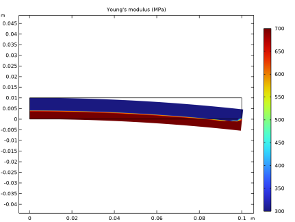
In the Settings window for Surface, click Replace Expression in the upper-right corner of the Expression section. From the menu, choose Component 1 (comp1) > Solid Mechanics > Material properties > solid.E - Young’s modulus - Pa.
|
|
3
|
|
4
|
|
5
|
|
6
|
|
1
|
|
2
|
Click
|
|
1
|
|
2
|
|
3
|
|
4
|
|
1
|
|
2
|
|
3
|
|
1
|
|
2
|
|
3
|
|
4
|
|
5
|