PDF

Vibration of a Squeezed Plate
Introduction
This model illustrates how to perform eigenfrequency and frequency response analyses for a contact problem.
A circular plate is squeezed between two thicker plates. The peak of a frequency response analysis is compared with the eigenfrequency and also with the natural frequency of an ideal case, that is, an annular plate fixed at the inner ring boundary.
Model Definition
The analysis is done using an assumption of 2D axisymmetry. The geometry is shown in Figure 1. A circular plate made of steel is constrained by means of mechanical contact with a holder modeled as two clamping plates.
Figure 1: Geometry consisting of a large thin plate clamped between two thicker plates.
Results and Discussion
For the plate holder radius ri = 0.2 m, the first natural frequency and the corresponding eigenmode are shown in Figure 2. The eigenfrequency is complex valued because of the damping added to model. The real part of the eigenfrequency is approximately 24.3 Hz. For an equivalent annular plate fixed at the inner ring boundary, the first natural frequency is around 25.2 Hz.
Figure 2: The first eigenmode for a plate clamped using contact. The plate holder radius is 0.2 m.
The frequency response for a frequency range containing the first eigenmode is shown in Figure 3.
Figure 3: Vertical displacement of the plate outer edge.
The maximum displacement occurs at a frequency value close to the eigenfrequency. The corresponding deformation of the plate is shown in Figure 4.
Figure 4: Response of the plate to a boundary load excitation at a frequency close to the first eigenfrequency.
The variation in the first natural frequency with respect to a change in the plate holder radius is shown in Figure 5. The results computed by means of the frequency domain analysis present a very good estimate of the eigenfrequency.
Figure 5: The first natural frequency as a function of the plate holder radius. The curves represent the results from the eigenfrequency analysis (annular constrained and squeezed plate) and from the maximum frequency response, respectively.
Notes About the COMSOL Implementation
The contact state is modeled via a stationary study step using the augmented Lagrangian method. The results are then used as a linearization point for both the eigenfrequency and the frequency domain study steps.
Application Library path: Structural_Mechanics_Module/Contact_and_Friction/squeezed_plate_response
Modeling Instructions
From the File menu, choose New.
New
In the New window, click  Model Wizard.
Model Wizard
1
In the Model Wizard window, click  2D Axisymmetric.
2
In the Select Physics tree, select Structural Mechanics > Solid Mechanics (solid).
3
Click Add.
4
Click  Study.
5
In the Select Study tree, select General Studies > Eigenfrequency.
6
Global Definitions
Parameters 1
1
In the Model Builder window, under Global Definitions click Parameters 1.
2
In the Settings window for Parameters, locate the Parameters section.
3
Geometry 1
Rectangle 1 (r1)
1
In the Geometry toolbar, click  Rectangle.
2
In the Settings window for Rectangle, locate the Size and Shape section.
3
In the Width text field, type r0.
4
In the Height text field, type th.
5
In the Width text field, type ro.
6
Click to expand the Layers section. In the table, enter the following settings:
7
Select the Layers to the left checkbox.
8
Clear the Layers on bottom checkbox.
9
Click  Build Selected.
Rectangle 2 (r2)
1
In the Geometry toolbar, click  Rectangle.
2
In the Settings window for Rectangle, locate the Size and Shape section.
3
In the Width text field, type ri.
4
In the Height text field, type 2*th.
5
Locate the Position section. In the z text field, type th.
Rectangle 3 (r3)
1
Right-click Rectangle 2 (r2) and choose Duplicate.
2
In the Settings window for Rectangle, locate the Position section.
3
In the z text field, type -2*th.
Form Union (fin)
Since only small sliding between the plates is expected, you can build the geometry with a union operation and use the Interior Contact node in the Solid Mechanics interface to model contact between internal boundaries.
1
In the Geometry toolbar, click  Build All.
Add Material
1
In the Materials toolbar, click  Add Material to open the Add Material window.
2
Go to the Add Material window.
3
In the tree, select Built-in > Structural steel.
4
Right-click and choose Add to Component 1 (comp1).
5
In the Materials toolbar, click  Add Material to close the Add Material window.
Solid Mechanics (solid)
Interior Contact 1
1
In the Physics toolbar, click  Boundaries and choose Interior Contact.
2
Use the Augmented Lagrangian method to increase the accuracy of the contact pressure.
3
In the Settings window for Interior Contact, locate the Contact Method section.
4
From the list, choose Augmented Lagrangian.
5
Locate the Contact Pressure Penalty Factor section. From the Tuned for list, choose Speed.
Roller 1
1
In the Physics toolbar, click  Boundaries and choose Roller.
2
Prescribed Displacement 1
1
In the Physics toolbar, click  Boundaries and choose Prescribed Displacement.
2
3
In the Settings window for Prescribed Displacement, locate the Prescribed Displacement section.
4
From the Displacement in z direction list, choose Prescribed.
5
In the u0z text field, type -1[um].
Linear Elastic Material 1
In the Model Builder window, click Linear Elastic Material 1.
Damping 1
1
In the Physics toolbar, click  Attributes and choose Damping.
2
In the Settings window for Damping, locate the Damping Settings section.
3
From the Damping type list, choose Isotropic loss factor.
Materials
Structural steel (mat1)
1
In the Model Builder window, under Component 1 (comp1) > Materials click Structural steel (mat1).
2
In the Settings window for Material, locate the Material Contents section.
3
Solid Mechanics (solid)
Fixed Constraint 1
1
In the Physics toolbar, click  Domains and choose Fixed Constraint.
2
This constraint makes the geometry equivalent to an annular plate fixed at the inner ring boundary.
Mesh 1
Mapped 1
In the Mesh toolbar, click  Mapped.
Distribution 1
1
Right-click Mapped 1 and choose Distribution.
2
3
In the Settings window for Distribution, locate the Distribution section.
4
In the Number of elements text field, type 4.
Distribution 2
1
In the Model Builder window, right-click Mapped 1 and choose Distribution.
2
3
In the Settings window for Distribution, locate the Distribution section.
4
In the Number of elements text field, type 24.
Size
1
In the Model Builder window, under Component 1 (comp1) > Mesh 1 click Size.
2
In the Settings window for Size, locate the Element Size section.
3
From the Predefined list, choose Extremely fine.
4
Click  Build All.
Study 1
1
In the Model Builder window, click Study 1.
2
In the Settings window for Study, locate the Study Settings section.
3
Clear the Generate default plots checkbox.
Step 1: Eigenfrequency
1
In the Model Builder window, under Study 1 click Step 1: Eigenfrequency.
2
In the Settings window for Eigenfrequency, locate the Study Settings section.
3
Select the Desired number of eigenfrequencies checkbox. In the associated text field, type 1.
4
In the Study toolbar, click  Compute.
Results
Add a plot of the mode shape from Result Templates.
Result Templates
1
In the Results toolbar, click  Result Templates to open the Result Templates window.
2
Go to the Result Templates window.
3
In the tree, select Study 1/Solution 1 (sol1) > Solid Mechanics > Mode Shape, 3D (solid).
4
Click the Add Result Template button in the window toolbar.
5
In the Results toolbar, click  Result Templates to close the Result Templates window.
Results
Mode Shape, Fixed
In the Settings window for 3D Plot Group, type Mode Shape, Fixed in the Label text field. The value of the real part should be close to 25.2 Hz.
Add Study
Next, compute the first natural frequency for a plate clamped by using contact.
1
In the Home toolbar, click  Add Study to open the Add Study window.
2
Go to the Add Study window.
3
Find the Studies subsection. In the Select Study tree, select Preset Studies for Selected Physics Interfaces > Eigenfrequency, Prestressed.
4
5
In the Home toolbar, click  Add Study to close the Add Study window.
Study 2
Step 1: Stationary
1
In the Settings window for Stationary, locate the Physics and Variables Selection section.
2
Select the Modify model configuration for study step checkbox.
3
In the tree, select Component 1 (comp1) > Solid Mechanics (solid), Controls spatial frame > Fixed Constraint 1.
4
Click  Disable.
Step 2: Eigenfrequency
1
In the Model Builder window, click Step 2: Eigenfrequency.
2
In the Settings window for Eigenfrequency, locate the Study Settings section.
3
Select the Desired number of eigenfrequencies checkbox. In the associated text field, type 1.
4
Locate the Physics and Variables Selection section. Select the Modify model configuration for study step checkbox.
5
In the tree, select Component 1 (comp1) > Solid Mechanics (solid), Controls spatial frame > Fixed Constraint 1.
6
Click  Disable.
7
In the Model Builder window, click Study 2.
8
In the Settings window for Study, locate the Study Settings section.
9
Clear the Generate default plots checkbox.
10
In the Study toolbar, click  Compute.
Result Templates
1
In the Results toolbar, click  Result Templates to open the Result Templates window.
2
Go to the Result Templates window.
3
In the tree, select Study 2/Solution 2 (sol2) > Solid Mechanics > Mode Shape, 3D (solid).
4
Click the Add Result Template button in the window toolbar.
5
In the Results toolbar, click  Result Templates to close the Result Templates window.
Results
Mode Shape, Prestressed
In the Settings window for 3D Plot Group, type Mode Shape, Prestressed in the Label text field. The value of the real part should be close to 24.3 Hz, which is slightly lower than for the fixed annular plate.
Solid Mechanics (solid)
Next, prepare to perform a frequency response analysis.
Boundary Load 1
1
In the Physics toolbar, click  Boundaries and choose Boundary Load.
2
3
In the Settings window for Boundary Load, locate the Force section.
4
Specify the fA vector as
5
Right-click Boundary Load 1 and choose Harmonic Perturbation.
Global Definitions
Parameters 1
1
In the Model Builder window, under Global Definitions click Parameters 1.
2
In the Settings window for Parameters, locate the Parameters section.
3
Add Study
1
In the Home toolbar, click  Add Study to open the Add Study window.
2
Go to the Add Study window.
3
Find the Studies subsection. In the Select Study tree, select Preset Studies for Selected Physics Interfaces > Frequency Domain, Prestressed.
4
5
In the Home toolbar, click  Add Study to close the Add Study window.
Study 3
Step 1: Stationary
1
In the Settings window for Stationary, locate the Physics and Variables Selection section.
2
Select the Modify model configuration for study step checkbox.
3
In the tree, select Component 1 (comp1) > Solid Mechanics (solid), Controls spatial frame > Fixed Constraint 1.
4
Click  Disable.
Step 2: Frequency-Domain Perturbation
Compute the solution for a frequency range that contains the reference frequency.
1
In the Model Builder window, click Step 2: Frequency-Domain Perturbation.
2
In the Settings window for Frequency-Domain Perturbation, locate the Study Settings section.
3
In the Frequencies text field, type freq_ref*range(0.95,5e-3,1.05).
4
Locate the Physics and Variables Selection section. Select the Modify model configuration for study step checkbox.
5
In the tree, select Component 1 (comp1) > Solid Mechanics (solid), Controls spatial frame > Fixed Constraint 1.
6
Click  Disable.
7
In the Model Builder window, click Study 3.
8
In the Settings window for Study, locate the Study Settings section.
9
Clear the Generate default plots checkbox.
10
In the Study toolbar, click  Compute.
Results
For comparison with the previously computed eigenmodes, modify the predefined stress plot to show the displacement at the reference frequency.
Result Templates
1
In the Results toolbar, click  Result Templates to open the Result Templates window.
2
Go to the Result Templates window.
3
In the tree, select Study 3/Solution 4 (sol4) > Solid Mechanics > Stress, 3D (solid).
4
Click the Add Result Template button in the window toolbar.
5
In the Results toolbar, click  Result Templates to close the Result Templates window.
Results
Displacement, Frequency Response
1
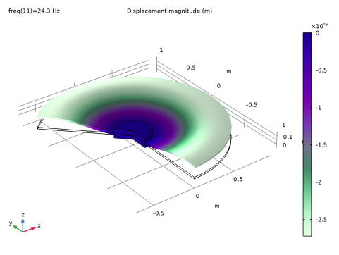
In the Settings window for 3D Plot Group, type Displacement, Frequency Response in the Label text field.
2
Locate the Data section. From the Parameter value (freq (Hz)) list, choose 24.3.
Surface 1
1
In the Model Builder window, expand the Displacement, Frequency Response node, then click Surface 1.
2
In the Settings window for Surface, locate the Expression section.
3
In the Expression text field, type solid.disp.
4
Locate the Coloring and Style section. From the Color table list, choose AuroraBorealis.
5
In the Displacement, Frequency Response toolbar, click  Plot.
Result Templates
The contact forces at the linearization point can be inspected by adding a plot from Result Templates.
1
In the Results toolbar, click  Result Templates to open the Result Templates window.
2
Go to the Result Templates window.
3
In the tree, select Study 2/Solution Store 1 (sol3) > Solid Mechanics > Contact Forces (solid).
4
Click the Add Result Template button in the window toolbar.
5
In the Results toolbar, click  Result Templates to close the Result Templates window.
Results
Contact Forces (solid)
In the Contact Forces (solid) toolbar, click  Plot.
Displacement Amplitude
Create a frequency response curve of the displacement amplitude at a point on the outer edge of the plate.
1
In the Results toolbar, click  1D Plot Group.
2
In the Settings window for 1D Plot Group, type Displacement Amplitude in the Label text field.
3
Locate the Data section. From the Dataset list, choose Study 3/Solution 4 (sol4).
4
Locate the Plot Settings section.
5
Select the x-axis label checkbox. In the associated text field, type Frequency (Hz).
6
Select the y-axis label checkbox. In the associated text field, type Displacement amplitude (mm).
Point Graph 1
1
Right-click Displacement Amplitude and choose Point Graph.
2
3
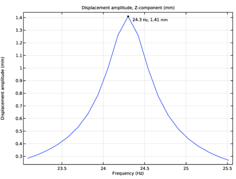
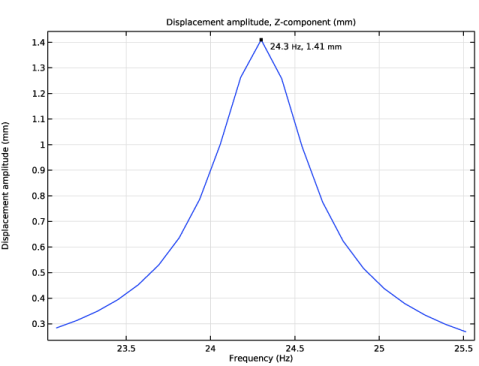
In the Settings window for Point Graph, click Replace Expression in the upper-right corner of the y-Axis Data section. From the menu, choose Component 1 (comp1) > Solid Mechanics > Displacement > Displacement amplitude (material and geometry frames) - m > solid.uAmpZ - Displacement amplitude, Z-component.
4
Locate the y-Axis Data section. From the Unit list, choose mm.
Graph Marker 1
1
Right-click Point Graph 1 and choose Graph Marker.
2
In the Settings window for Graph Marker, locate the Display section.
3
From the Display list, choose Max.
4
Locate the Text Format section. Select the Show x-coordinate checkbox.
5
Select the Include unit checkbox.
6
In the Precision text field, type 3.
7
In the Displacement Amplitude toolbar, click  Plot.
Study 1
Next, extend all studies with a Parametric Sweep to study how the radius of the clamping plate ri affects the natural frequency of the plate.
Parametric Sweep
1
In the Study toolbar, click  Parametric Sweep.
2
In the Settings window for Parametric Sweep, locate the Study Settings section.
3
4
5
In the Study toolbar, click  Compute.
Results
Add an Evaluation Group to extract the natural frequency.
Eigenfrequencies, Fixed
1
In the Results toolbar, click  Evaluation Group.
2
In the Settings window for Evaluation Group, type Eigenfrequencies, Fixed in the Label text field.
3
Locate the Data section. From the Dataset list, choose Study 1/Parametric Solutions 1 (sol6).
4
Click to expand the Format section. From the Include parameters list, choose Off.
Global Evaluation 1
1
Right-click Eigenfrequencies, Fixed and choose Global Evaluation.
2
In the Settings window for Global Evaluation, locate the Expressions section.
3
4
In the Eigenfrequencies, Fixed toolbar, click  Evaluate.
Study 2
Parametric Sweep
1
In the Study toolbar, click  Parametric Sweep.
2
In the Settings window for Parametric Sweep, locate the Study Settings section.
3
4
5
In the Study toolbar, click  Compute.
Results
Eigenfrequencies, Prestressed
1
In the Model Builder window, right-click Eigenfrequencies, Fixed and choose Duplicate.
2
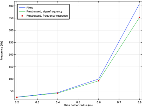
In the Settings window for Evaluation Group, type Eigenfrequencies, Prestressed in the Label text field.
3
Locate the Data section. From the Dataset list, choose Study 2/Parametric Solutions 2 (sol11).
4
In the Eigenfrequencies, Prestressed toolbar, click  Evaluate.
Global Definitions
In order to add a parametric sweep to the prestressed frequency response study, we first need to redefine the reference frequency freq_ref using an interpolation function to capture the change in natural frequency with the holder plate radius.
Interpolation 1 (int1)
1
In the Home toolbar, click  Functions and choose Global > Interpolation.
2
In the Settings window for Interpolation, locate the Definition section.
3
From the Data source list, choose Result table.
4
From the Table from list, choose Eigenfrequencies, Prestressed.
5
Locate the Data Column Settings section. In the table, click to select the cell at row number 1 and column number 1.
6
In the Unit text field, type m.
7
8
In the Name text field, type freq_ref.
9
In the Unit text field, type Hz.
10
Locate the Interpolation and Extrapolation section. From the Interpolation list, choose Nearest neighbor.
Parameters 1
1
In the Model Builder window, click Parameters 1.
2
In the Settings window for Parameters, locate the Parameters section.
3
Study 3
Parametric Sweep
1
In the Study toolbar, click  Parametric Sweep.
2
In the Settings window for Parametric Sweep, locate the Study Settings section.
3
4
5
In the Study toolbar, click  Compute.
Results
Displacement Amplitude
1
In the Model Builder window, under Results click Displacement Amplitude.
2
In the Settings window for 1D Plot Group, locate the Data section.
3
From the Dataset list, choose Study 3/Parametric Solutions 3 (sol16).
Point Graph 1
1
In the Model Builder window, click Point Graph 1.
2
In the Settings window for Point Graph, click to expand the Legends section.
3
Select the Show legends checkbox.
4
Find the Include subsection. Clear the Point checkbox.
5
In the Displacement Amplitude toolbar, click  Plot.
Eigenfrequencies, Frequency Response
Finally, create a plot to show the dependence of the natural frequency on ri for the three studies. First, find the frequency that yields the maximum displacement amplitude in the prestressed frequency response study.
1
In the Results toolbar, click  Evaluation Group.
2
In the Settings window for Evaluation Group, type Eigenfrequencies, Frequency Response in the Label text field.
3
Locate the Data section. From the Dataset list, choose Study 3/Parametric Solutions 3 (sol16).
4
Locate the Format section. From the Include parameters list, choose Off.
5
From the Concatenation list, choose Vertical.
Point Evaluation 1
1
Right-click Eigenfrequencies, Frequency Response and choose Point Evaluation.
2
In the Settings window for Point Evaluation, locate the Data section.
3
From the Dataset list, choose Study 3/Parametric Solutions 3 (sol16).
4
From the Parameter selection (ri) list, choose From list.
5
In the Parameter values (ri (m)) list box, select 0.2.
6
7
Locate the Expressions section. In the table, enter the following settings:
8
Locate the Data Series Operation section. From the Transformation list, choose Maximum.
9
Select the Include parameters checkbox.
10
In the Eigenfrequencies, Frequency Response toolbar, click  Evaluate.
Point Evaluation 2
1
Right-click Point Evaluation 1 and choose Duplicate.
2
In the Settings window for Point Evaluation, locate the Data section.
3
In the Parameter values (ri (m)) list box, select 0.4.
Point Evaluation 3
1
Right-click Point Evaluation 2 and choose Duplicate.
2
In the Settings window for Point Evaluation, locate the Data section.
3
In the Parameter values (ri (m)) list box, select 0.6.
Point Evaluation 4
1
Right-click Point Evaluation 3 and choose Duplicate.
2
In the Settings window for Point Evaluation, locate the Data section.
3
In the Parameter values (ri (m)) list box, select 0.8.
Eigenfrequencies, Frequency Response
1
In the Model Builder window, click Eigenfrequencies, Frequency Response.
2
In the Eigenfrequencies, Frequency Response toolbar, click  Evaluate.
Natural Frequencies
Use the data in the three Evaluation Groups to plot the natural frequency as a function of the plate holder radius using Table Graphs.
1
In the Results toolbar, click  1D Plot Group.
2
In the Settings window for 1D Plot Group, type Natural Frequencies in the Label text field.
3
Locate the Data section. From the Dataset list, choose None.
4
Locate the Legend section. From the Position list, choose Upper left.
Eigenfrequencies, Fixed
1
Right-click Natural Frequencies and choose Table Graph.
2
In the Settings window for Table Graph, locate the Data section.
3
From the Source list, choose Evaluation group.
4
In the Label text field, type Eigenfrequencies, Fixed.
5
Click to expand the Legends section. Select the Show legends checkbox.
6
From the Legends list, choose Manual.
7
Eigenfrequencies, Prestressed
1
Right-click Eigenfrequencies, Fixed and choose Duplicate.
2
In the Settings window for Table Graph, type Eigenfrequencies, Prestressed in the Label text field.
3
Locate the Data section. From the Evaluation group list, choose Eigenfrequencies, Prestressed.
4
Locate the Legends section. In the table, enter the following settings:
Eigenfrequencies, Frequency Response
1
Right-click Eigenfrequencies, Prestressed and choose Duplicate.
2
In the Settings window for Table Graph, type Eigenfrequencies, Frequency Response in the Label text field.
3
Locate the Data section. From the x-axis data list, choose Plate holder radius (m).
4
From the Plot columns list, choose Manual.
5
In the Columns list box, select Frequency (Hz).
6
Locate the Coloring and Style section. Find the Line style subsection. From the Line list, choose None.
7
Find the Line markers subsection. From the Marker list, choose Point.
8
Locate the Legends section. In the table, enter the following settings:
9
In the Natural Frequencies toolbar, click  Plot.