PDF

Seismic Event, Explicit Dynamics
Introduction
This tutorial studies the evolution of seismic waves in a two-dimensional isotropic linear elastic half space with a small mountain on its top. The seismic event is due to a vertical load applied at a point on the top of the half space to the right of the mountain. As a result of the applied load, various types of elastic waves propagate into the bulk and along the top surface. In particular, these include longitudinal, shear, and head (von Schmidt) waves, as well as Rayleigh waves.
The mountain acts as a scatterer, which results in a new envelope of backscattering waves of the same nature.
This is a version of the model Ground Motion After Seismic Event: Scattering off a Small Mountain, where a Solid Mechanics, Explicit Dynamics interface is used instead of the Elastic Waves, Time Explicit interface.
Model Definition
The half space y < 0 with a small mountain on its top is made of a linear elastic material with the properties given in Table 1.
ρ
cp
cs
The mountain has the height of 200 m. Its shape is given by a Gaussian bell
 km
located 5 km to the left of the vertical line y = 0. The geometry repeats the one used in Ref. 1.
The half space is modeled as a 40 km wide and 20 km high rectangle with the center of its top side placed at the origin (0, 0).
The reflections of the waves at the outer boundaries are suppressed by adding a Low-Reflecting Boundary condition to the sides and bottom of the rectangle.
The top of the half space is free, except for the load at the point (0, 0). Its distribution in time is given by a Ricker wavelet shown in Figure 1.
Figure 1: Source distribution in time.
The free top boundary is of particular interest, because it gives rise to Rayleigh waves that propagate near the surface with a speed lower than that of the shear wave in the bulk material. One of the classical estimates of the Rayleigh wave speed, vR, with respect to the shear wave speed is given by
where ν is the Poisson’s ratio. It is therefore important to use the Rayleigh wave speed while building the mesh in order to resolve the Rayleigh waves properly. That is, the minimum wavelength used to define the maximum mesh element size will be
Results and Discussion
Figure 2 shows the velocity magnitude profiles in the physical domain computed at 3, 6, 9, and 12 s. In the upper-left figure, the propagation of the pressure (faster) and the shear (slower) waves are shown at t = 3 s.
When the wave front reaches the mountain, it results in the backscattering of the waves. This is seen in the upper-right picture (t = 6 s). The Rayleigh wave also becomes distinguishable in the region below the surface, as it travels slower than the shear wave. The head (von Schmidt) wave that has a conical shape and propagates at the critical angle β to the ground top, such that sinβ = cs/cp is also visible.
In the lower-left and lower-right pictures (t = 9 s and t = 12 s), the initial wave front and the scattered waves leave the computational domain.
Figure 2: Velocity magnitude profiles at four different time steps
The second principal invariant of the stress tensor contains information on the pressure and shear waves traveling through the solid. Pressure waves have a positive value of this stress invariant, while shear waves show a negative value. As this invariant has units of squared stress, we take the square root of the absolute value of the invariant and multiply it with its sign to create Figure 3.
Figure 3: Signed squared root of the second principal invariant at four different time steps.
Pressure waves are colored in blue, while shear, Rayleigh, and head waves are colored in orange.
Notes About the COMSOL Implementation
To resolve the Rayleigh wave properly the maximum element size is computed as the minimum wavelength divided by 10 since linear elements are used in the Solid Mechanics, Explicit Dynamics interface.
Reference
1. D. Appelö and N.A. Petersson, “A Stable Finite Difference Method for the Elastic Wave Equation on Complex Geometries with Free Surfaces,” Commun. Comput. Phys., vol. 5, pp. 84–107, 2009.
Application Library path: Structural_Mechanics_Module/Elastic_Waves/seismic_event
Modeling Instructions
From the File menu, choose New.
New
In the New window, click  Model Wizard.
Model Wizard
1
In the Model Wizard window, click  2D.
2
In the Select Physics tree, select Structural Mechanics > Explicit Dynamics > Solid Mechanics, Explicit Dynamics (solid).
3
Click Add.
4
Click  Study.
5
In the Select Study tree, select Preset Studies for Selected Physics Interfaces > Explicit Dynamics.
6
Global Definitions
Parameters 1
1
In the Model Builder window, under Global Definitions click Parameters 1.
2
In the Settings window for Parameters, locate the Parameters section.
3
Click  Load from File.
4
Create the source space and time functions given by a Gaussian and a Ricker wavelet, respectively.
G_space
1
In the Home toolbar, click  Functions and choose Global > Analytic.
2
In the Settings window for Analytic, type G_space in the Label text field.
3
In the Function name text field, type G_space.
4
Locate the Definition section. In the Expression text field, type 1/sqrt(pi*dS)*exp(-x^2/dS).
5
Locate the Units section. In the table, enter the following settings:
6
In the Function text field, type 1.
G_time
1
In the Home toolbar, click  Functions and choose Global > Analytic.
2
In the Settings window for Analytic, type G_time in the Label text field.
3
In the Function name text field, type G_time.
4
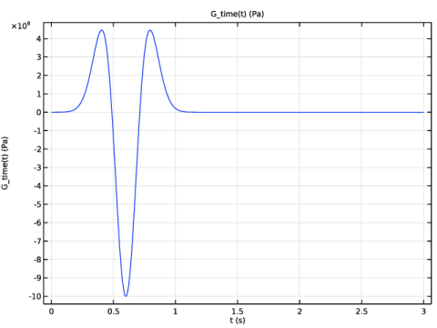
Locate the Definition section. In the Expression text field, type 1e9*(2*(pi*f0*(t - t0))^2 - 1)*exp(-(pi*f0*(t - t0))^2).
5
In the Arguments text field, type t.
6
Locate the Units section. In the table, enter the following settings:
7
In the Function text field, type Pa.
8
Locate the Plot Parameters section. In the table, enter the following settings:
9
Click  Create Plot.
Results
Impulse Frequency Content
1
In the Settings window for 1D Plot Group, type Impulse Frequency Content in the Label text field.
2
Click to expand the Title section. From the Title type list, choose Manual.
3
In the Title text area, type FFT of G_time (Pa).
4
Locate the Plot Settings section.
5
Select the y-axis label checkbox. In the associated text field, type FFT of the signal.
Function 1
1
In the Model Builder window, expand the Impulse Frequency Content node, then click Function 1.
2
In the Settings window for Function, locate the Output section.
3
From the Display list, choose Discrete Fourier transform.
4
From the Show list, choose Frequency spectrum.
5
From the Scale list, choose Multiply by sampling period.
6
In the Impulse Frequency Content toolbar, click  Plot.
7
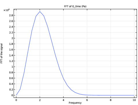
Select the Frequency range checkbox.
8
In the Maximum text field, type 10.
9
In the Impulse Frequency Content toolbar, click  Plot.
The Fourier transformation of the signal should look like this. The plot indicates that the mesh should resolve frequency content up to 4 to 5 Hz.
Geometry 1
The geometry sequence for the model is available in a file. If you want to create it from scratch yourself, you can follow the instructions in the Geometry Modeling Instructions section. Otherwise, insert the geometry sequence as follows:
1
In the Geometry toolbar, click Insert Sequence and choose Insert Sequence.
2
3
In the Geometry toolbar, click  Build All.
4
In the Model Builder window, under Component 1 (comp1) click Geometry 1.
Materials
Ground Material
1
In the Model Builder window, under Component 1 (comp1) right-click Materials and choose Blank Material.
2
In the Settings window for Material, type Ground Material in the Label text field.
3
Click to expand the Material Properties section. In the Material properties tree, select Solid Mechanics > Linear Elastic Material > Pressure-Wave and Shear-Wave Speeds.
4
Click  Add to Material.
5
Locate the Material Contents section. In the table, enter the following settings:
Solid Mechanics, Explicit Dynamics (solid)
Linear Elastic Material 1
1
In the Model Builder window, expand the Component 1 (comp1) > Materials > Ground Material (mat1) node, then click Component 1 (comp1) > Solid Mechanics, Explicit Dynamics (solid) > Linear Elastic Material 1.
2
In the Settings window for Linear Elastic Material, locate the Quadrature Settings section.
3
Find the Hexahedron subsection. From the Hourglass stabilization list, choose Hessian.
Low-Reflecting Boundary 1
1
In the Physics toolbar, click  Boundaries and choose Low-Reflecting Boundary.
2
Boundary Load 1
1
In the Physics toolbar, click  Boundaries and choose Boundary Load.
2
3
In the Settings window for Boundary Load, locate the Force section.
4
Specify the fA vector as
Mesh 1
Build the mesh specifying the maximum element size.
Free Quad 1
1
In the Mesh toolbar, click  Free Quad.
2
In the Settings window for Free Quad, locate the Domain Selection section.
3
From the Geometric entity level list, choose Domain.
4
5
Click to expand the Control Entities section. From the Smooth across removed control entities list, choose Off.
6
Click to expand the Mesh Generation section. From the Method list, choose Quad.
Size 1
Right-click Free Quad 1 and choose Size.
Size
1
In the Settings window for Size, click to expand the Element Size Parameters section.
2
In the Maximum element size text field, type cr/(2*f0)/10.
3
In the Minimum element size text field, type cr/(2*f0)/10.
4
In the Maximum element growth rate text field, type 1.5.
5
In the Curvature factor text field, type 0.5.
Size 1
1
In the Model Builder window, under Component 1 (comp1) > Mesh 1 > Free Quad 1 click Size 1.
2
3
In the Settings window for Size, locate the Element Size section.
4
Click the Custom button.
Copy Domain 1
1
In the Model Builder window, right-click Mesh 1 and choose Copying Operations > Copy Domain.
2
3
In the Settings window for Copy Domain, locate the Destination Domains section.
4
Click to select the  Activate Selection toggle button.
5
6
Click to expand the Control Entities section. From the Smooth across removed control entities list, choose On.
Mapped 1
1
In the Mesh toolbar, click  Mapped.
2
In the Settings window for Mapped, click to expand the Control Entities section.
3
From the Smooth across removed control entities list, choose Off.
Study 1
1
In the Model Builder window, click Study 1.
2
In the Settings window for Study, locate the Study Settings section.
3
Clear the Generate default plots checkbox.
Step 1: Explicit Dynamics
1
In the Model Builder window, under Study 1 click Step 1: Explicit Dynamics.
2
In the Settings window for Explicit Dynamics, locate the Study Settings section.
3
In the Output times text field, type range(0,1,12).
4
Click to expand the Results While Solving section. From the Update at list, choose Time steps taken by solver.
5
In the Study toolbar, click  Compute.
Results
Preferred Units 1
1
In the Results toolbar, click  Configurations and choose Preferred Units.
2
In the Settings window for Preferred Units, locate the Units section.
3
Click  Add Physical Quantity.
4
In the Physical Quantity dialog, type pre in the text field.
5
In the tree, select General > Pressure (Pa).
6
7
In the Settings window for Preferred Units, locate the Units section.
8
9
Select the Apply conversions to expressions with the same dimensions checkbox.
10
Click  Apply.
Velocity
1
In the Results toolbar, click  2D Plot Group.
2
In the Settings window for 2D Plot Group, type Velocity in the Label text field.
3
Locate the Data section. From the Time (s) list, choose 3.
4
Click to expand the Selection section. From the Geometric entity level list, choose Domain.
5
6
Select the Apply to dataset edges checkbox.
7
Locate the Plot Settings section. From the Frame list, choose Spatial  (x, y, z).
Surface 1
1
Right-click Velocity and choose Surface.
2
In the Settings window for Surface, locate the Expression section.
3
In the Expression text field, type solid.vel.
4
Click to expand the Range section. Select the Manual color range checkbox.
5
In the Maximum text field, type 0.5.
These settings will sharpen the contrast of the velocity profile.
6
Locate the Coloring and Style section. From the Color table list, choose Viridis.
7
From the Color table transformation list, choose Reverse.
8
Click to expand the Quality section. From the Evaluation settings list, choose Manual.
9
From the Smoothing list, choose Everywhere.
Then generate the plots at 6, 9, and 12 s. The structural velocity profiles at the time steps chosen in Study 1 are shown in Figure 2.
Pressure
1
In the Results toolbar, click  2D Plot Group.
2
In the Settings window for 2D Plot Group, type Pressure in the Label text field.
3
Locate the Data section. From the Time (s) list, choose 6.
4
Locate the Selection section. From the Geometric entity level list, choose Domain.
5
6
Select the Apply to dataset edges checkbox.
Surface 1
1
Right-click Pressure and choose Surface.
2
In the Settings window for Surface, locate the Expression section.
3
In the Expression text field, type solid.pmGp.
4
Locate the Range section. Select the Manual color range checkbox.
5
In the Minimum text field, type -0.25.
6
In the Maximum text field, type 0.25.
7
Locate the Coloring and Style section. From the Color table list, choose Dipole.
8
From the Scale list, choose Linear symmetric.
9
Locate the Quality section. From the Evaluation settings list, choose Manual.
10
In the Pressure toolbar, click  Plot.
Create the last plot that will help discern the pressure and shear waves.
Pressure and Shear Waves
1
In the Results toolbar, click  2D Plot Group.
2
In the Settings window for 2D Plot Group, type Pressure and Shear Waves in the Label text field.
3
Locate the Data section. From the Time (s) list, choose 3.
4
Locate the Selection section. From the Geometric entity level list, choose Domain.
5
6
Select the Apply to dataset edges checkbox.
7
Click to expand the Title section. From the Title type list, choose Label.
8
Locate the Color Legend section. Select the Show units checkbox.
9
Click to expand the Quality section. From the Smoothing list, choose Inside geometry domains.
Surface 1
1
Right-click Pressure and Shear Waves and choose Surface.
2
In the Settings window for Surface, locate the Expression section.
3
In the Expression text field, type solid.gpeval(sqrt(abs(solid.I2s))*sign(solid.I2s)).
4
Locate the Range section. Select the Manual color range checkbox.
5
In the Minimum text field, type -0.24.
6
In the Maximum text field, type 0.3.
7
Locate the Coloring and Style section. From the Color table list, choose Twilight.
8
Locate the Quality section. From the Evaluation settings list, choose Manual.
9
From the Resolution list, choose No refinement.
10
From the Smoothing list, choose Everywhere.
11
In the Pressure and Shear Waves toolbar, click  Plot.
Loop through the different times to reproduce Figure 3.
Animation 1
1
In the Results toolbar, click  Animation and choose Player.
2
In the Settings window for Animation, locate the Scene section.
3
From the Subject list, choose Pressure and Shear Waves.
4
Locate the Frames section. In the Number of frames text field, type 13.
5
In the Frame number text field, type 13.
Geometry Modeling Instructions
From the File menu, choose New.
New
In the New window, click  Blank Model.
Add Component
In the Home toolbar, click  Add Component and choose 2D.
Geometry 1
1
In the Settings window for Geometry, locate the Units section.
2
From the Length unit list, choose km.
Rectangle 1 (r1)
1
In the Geometry toolbar, click  Rectangle.
2
In the Settings window for Rectangle, locate the Size and Shape section.
3
In the Width text field, type 40[km].
4
In the Height text field, type 20[km].
5
Locate the Position section. In the x text field, type -20[km].
6
In the y text field, type -20[km].
7
Click to expand the Layers section. Select the Layers to the left checkbox.
8
Select the Layers to the right checkbox.
9
Parametric Curve 1 (pc1)
1
In the Geometry toolbar, click  More Primitives and choose Parametric Curve.
2
In the Settings window for Parametric Curve, locate the Parameter section.
3
In the Maximum text field, type 2[km].
4
Locate the Expressions section. In the x text field, type s.
5
In the y text field, type 0.2*(exp(-((s - 1[km])/0.3[km])^2) - exp(-(1[km]/ 0.3[km])^2))[km].
6
Locate the Position section. In the x text field, type -6[km].
7
Click  Build Selected.
Rectangle 2 (r2)
1
In the Geometry toolbar, click  Rectangle.
2
In the Settings window for Rectangle, locate the Size and Shape section.
3
In the Width text field, type 2.4[km].
4
In the Height text field, type 0.7[km].
5
Locate the Position section. In the x text field, type -6.2[km].
Point 1 (pt1)
1
In the Geometry toolbar, click  Point.
2
In the Settings window for Point, click  Build Selected.
Partition Objects 1 (par1)
1
In the Geometry toolbar, click  Booleans and Partitions and choose Partition Objects.
2
3
In the Settings window for Partition Objects, locate the Partition Objects section.
4
Click to select the  Activate Selection toggle button for Tool objects.
5
6
Click  Build Selected.
Delete Entities 1 (del1)
1
In the Model Builder window, right-click Geometry 1 and choose Delete Entities.
2
In the Settings window for Delete Entities, locate the Entities or Objects to Delete section.
3
From the Geometric entity level list, choose Domain.
4
On the object par1, select Domain 1 only.
5
Click  Build Selected.
Fillet 1 (fil1)
1
In the Geometry toolbar, click  Fillet.
2
On the object r1, select Points 1 and 10 only.
3
In the Settings window for Fillet, locate the Radius section.
4
In the Radius text field, type 1.
5
Click  Build Selected.
Next create additional domains to improve the mesh quality at the corners.
Polygon 1 (pol1)
1
In the Geometry toolbar, click  Polygon.
2
In the Settings window for Polygon, locate the Object Type section.
3
From the Type list, choose Open curve.
4
Locate the Coordinates section. In the table, enter the following settings:
5
Click  Build Selected.
Polygon 2 (pol2)
1
In the Geometry toolbar, click  Polygon.
2
In the Settings window for Polygon, locate the Object Type section.
3
From the Type list, choose Open curve.
4
Locate the Coordinates section. In the table, enter the following settings:
5
Click  Build Selected.
Polygon 3 (pol3)
1
In the Geometry toolbar, click  Polygon.
2
In the Settings window for Polygon, locate the Object Type section.
3
From the Type list, choose Open curve.
4
Locate the Coordinates section. In the table, enter the following settings:
Mirror 1 (mir1)
1
In the Geometry toolbar, click  Transforms and choose Mirror.
2
In the Settings window for Mirror, locate the Input section.
3
Select the Keep input objects checkbox.
4
Select the objects pol1, pol2, and pol3 only.
5
Click  Build Selected.
Form Composite Domains 1 (cmd1)
1
In the Geometry toolbar, click  Virtual Operations and choose Form Composite Domains.
2
On the object fin, select Domains 7 and 8 only.
3
In the Settings window for Form Composite Domains, click  Build Selected.
Mesh Control Edges 1 (mce1)
1
In the Geometry toolbar, click  Virtual Operations and choose Mesh Control Edges.
2
On the object cmd1, select Boundaries 2, 6, 7, 9, 11, 22, and 26–29 only.
3
In the Settings window for Mesh Control Edges, click  Build Selected.