PDF

Roundness Evaluation of a Deformed Hole
Introduction
During manufacturing processes, or during use, the geometrical shape of structural parts can deviate from what was intended. For instance, a hole can deviate from an ideal circle. In an assembly, it can be important to measure and control this deviation. The process of obtaining this information is often called roundness (or circularity) error evaluation.
There are different methods to measure the roundness error, all based on optimization techniques:
This model illustrates how to reuse the deformed shape data for an optimization analysis to obtain the center coordinates and radii of the circles for each of the methods listed above.
Model Definition
In this model, a pressure load is applied to a plate with a hole in a first study. The boundary condition used are not important; the only purpose is to provide some non-trivial deformation. The hole does no longer remain circular.
Deformed shape data is then exported to a table. Finally, using this deformed shape data, the roundness error can be computed as the difference between the circles with the minimum and maximum radii that fit the deformed shape
To obtain the maximum circle radius and the minimum circle radius, five different techniques are considered here. The first one (LSQ) uses the predefined Least-Squares Fit function, which does not require a special solver to be used. The other four methods require an optimization solver and thus the Optimization Module. These four methods are described below.
Least Square Circle (LSC)
This method searches for the radius Rc and the center coordinates (xc, yc) of the circle that minimizes the sum of the square deviation from the points of the deformed shape. The objective function can be written as
Solving this problem, the minimum and maximum radii can be obtained as
Minimum Zone Circle (MZC)
This method directly minimizes the roundness error. Two concentric circles are assumed, one with the maximum radius that contains all points of the deformed shape, and the other with the smallest radius that is inscribed in the deformed shape. The objective function is then
Minimum Circumscribed Circle (MMC)
The MCC method searches for the circle with the smallest radius that is circumscribed around the deformed shape. The objective function is
Then minimum circle can be obtained as
Maximum Inscribed Circle (MIC)
The MIC method searches for the circle with the largest radius that inside the deformed shape. The objective function is
Then minimum circle can be obtained as
Results and Discussion
Figure 1 displays the von Mises stress distribution in the part for the assumed boundary condition. The stress concentration around the hole is a result of the ovalization of the hole.
Figure 1: von Mises stress distribution in the plate.
Figure 2 and Figure 3 show the deformed shape of the hole together with the minimum (in blue) and maximum (in green) circle. From top to bottom: the minimum circumscribed circle (MCC) method, the maximum inscribed circle (MIC) method, the Least-Squares Fit function (LSQ), the Least-Squares Circle (LSC) method, and the minimum zone circle (MZC) method.
Figure 2: The minimum (blue) and maximum (green) circle obtained using MCC and MIC methods.
Figure 3: The minimum (blue) and maximum (green) circle using LSQ, LSC, and MZC methods.
In the table Table 1 below you can see the coordinates of the center, the minimum and the maximum radii, and the roundness error (the difference between Rmax and Rmin). The solutions using the different methods differ slightly. The minimum zone circle (MZC) method provides the smallest roundness error. This is not surprising, since that method directly aims at minimizing the roundness error. This may be interpreted as the best result, but there is no unique answer to what is the best fit of the two circles.
Notes About the COMSOL Implementation
To use any of the optimization methods described in this model, you must be able to express the deformed shape as function of a local parameter. Here, the polar angle along the deformed edge is used. To export the deformed shape data along an edge to a table, you need to create a Cut Point 3D dataset combined with a solution dataset restricted to the edge of interest. With such a dataset, you can easily generate a table that has the columns populated with the angle position, the x-coordinates, and the y-coordinates along every point along the selected edge.
Application Library path: Structural_Mechanics_Module/Sensitivity_and_Optimization/roundness_evaluation
Modeling Instructions
From the File menu, choose New.
New
In the New window, click  Model Wizard.
Model Wizard
1
In the Model Wizard window, click  3D.
2
In the Select Physics tree, select Structural Mechanics > Solid Mechanics (solid).
3
Click Add.
4
Click  Study.
5
In the Select Study tree, select General Studies > Stationary.
6
Global Definitions
Parameters 1
1
In the Model Builder window, under Global Definitions click Parameters 1.
2
In the Settings window for Parameters, locate the Parameters section.
3
Geometry 1
Block 1 (blk1)
1
In the Geometry toolbar, click  Block.
2
In the Settings window for Block, locate the Size and Shape section.
3
In the Height text field, type 0.1.
Cylinder 1 (cyl1)
1
In the Geometry toolbar, click  Cylinder.
2
In the Settings window for Cylinder, locate the Size and Shape section.
3
In the Radius text field, type R0.
4
In the Height text field, type 0.1.
5
Locate the Position section. In the x text field, type x0.
6
In the y text field, type y0.
Difference 1 (dif1)
1
In the Geometry toolbar, click  Booleans and Partitions and choose Difference.
2
3
In the Settings window for Difference, locate the Difference section.
4
Click to select the  Activate Selection toggle button for Objects to subtract.
5
6
Click  Build Selected.
Form Union (fin)
1
In the Model Builder window, click Form Union (fin).
2
In the Settings window for Form Union/Assembly, click  Build Selected.
Add Material
1
In the Materials toolbar, click  Add Material to open the Add Material window.
2
Go to the Add Material window.
3
In the tree, select Built-in > Nylon.
4
Click the Add to Component button in the window toolbar.
5
In the Materials toolbar, click  Add Material to close the Add Material window.
Solid Mechanics (solid)
Fixed Constraint 1
1
In the Physics toolbar, click  Boundaries and choose Fixed Constraint.
2
Boundary Load 1
1
In the Physics toolbar, click  Boundaries and choose Boundary Load.
2
3
In the Settings window for Boundary Load, locate the Force section.
4
From the Load type list, choose Pressure.
5
In the p text field, type p.
Study 1
Step 1: Stationary
1
In the Model Builder window, under Study 1 click Step 1: Stationary.
2
In the Settings window for Stationary, locate the Study Settings section.
3
Select the Include geometric nonlinearity checkbox.
4
Click to expand the Study Extensions section. Select the Auxiliary sweep checkbox.
5
6
7
In the Study toolbar, click  Compute.
Results
Study 1/Solution 1 (2) (sol1)
1
In the Model Builder window, expand the Results > Datasets node.
2
Right-click Results > Datasets > Study 1/Solution 1 (sol1) and choose Duplicate.
Selection
1
In the Results toolbar, click  Attributes and choose Selection.
2
In the Settings window for Selection, locate the Geometric Entity Selection section.
3
From the Geometric entity level list, choose Edge.
4
Cut Point 3D 1
1
In the Results toolbar, click  Cut Point 3D.
2
In the Settings window for Cut Point 3D, locate the Data section.
3
From the Dataset list, choose Study 1/Solution 1 (2) (sol1).
4
Locate the Point Data section. From the Entry method list, choose Regular grid.
5
In the Number of X points text field, type 20.
6
In the Number of Y points text field, type 20.
7
In the Number of Z points text field, type 1.
8
From the Snapping list, choose Snap to closest edge.
9
Deformed Shape
1
In the Results toolbar, click  Evaluation Group.
2
In the Settings window for Evaluation Group, type Deformed Shape in the Label text field.
3
Locate the Data section. From the Dataset list, choose Cut Point 3D 1.
4
From the Parameter selection (p) list, choose Last.
5
Locate the Transformation section. Select the Transpose checkbox.
6
Click to expand the Format section. From the Include parameters list, choose Off.
7
From the Concatenation list, choose Vertical.
Point Evaluation 1
1
Right-click Deformed Shape and choose Point Evaluation.
2
In the Settings window for Point Evaluation, locate the Expressions section.
3
Point Evaluation 2
1
In the Model Builder window, right-click Deformed Shape and choose Point Evaluation.
2
In the Settings window for Point Evaluation, locate the Expressions section.
3
Point Evaluation 3
1
Right-click Deformed Shape and choose Point Evaluation.
2
In the Settings window for Point Evaluation, locate the Expressions section.
3
4
In the Deformed Shape toolbar, click  Evaluate.
Global Definitions
Interpolation 1 (int1)
1
In the Home toolbar, click  Functions and choose Global > Interpolation.
2
In the Settings window for Interpolation, locate the Definition section.
3
From the Data source list, choose Result table.
4
Locate the Data Column Settings section. In the table, click to select the cell at row number 2 and column number 2.
5
In the Unit text field, type m.
6
7
In the Name text field, type int2.
8
In the Unit text field, type m.
Parameters 1
1
In the Model Builder window, click Parameters 1.
2
In the Settings window for Parameters, locate the Parameters section.
3
Variables 1
1
In the Model Builder window, right-click Global Definitions and choose Variables.
2
In the Settings window for Variables, locate the Variables section.
3
Least-Squares Fit 1 (lsq1_fun1)
1
In the Home toolbar, click  Functions and choose Global > Least-Squares Fit.
2
In the Settings window for Least-Squares Fit, locate the Data section.
3
From the Data source list, choose Result table.
4
Locate the Data Column Settings section. In the table, enter the following settings:
5
6
Locate the Parameters section. In the table, enter the following settings:
7
Locate the Data Column Settings section. In the Expression text field, type xc+r*cos(x1).
8
In the Unit text field, type m.
9
10
In the Expression text field, type yc+r*sin(x1).
11
In the Unit text field, type m.
12
Click  Fit Parameters.
13
Click to expand the Plot Parameters section. Click  Plot.
14
From the Function name list, choose lsq1_fun2.
15
Variables 1
1
In the Model Builder window, click Variables 1.
2
In the Settings window for Variables, locate the Variables section.
3
4
Click the  Show More Options button in the Model Builder toolbar.
5
In the Show More Options dialog, select General > Variable Utilities in the tree.
6
7
Definitions
Expression Operator 1 (exop1)
1
In the Definitions toolbar, click  Variable Utilities and choose Expression Operator.
2
In the Settings window for Expression Operator, type dist in the Name text field.
3
Locate the Definition section. In the Expression text field, type sqrt((x1-x2)^2+(y1-y2)^2).
4
Maximum 1 (maxop1)
1
In the Definitions toolbar, click  Nonlocal Couplings and choose Maximum.
2
In the Settings window for Maximum, locate the Source Selection section.
3
From the Geometric entity level list, choose Edge.
4
Minimum 1 (minop1)
1
In the Definitions toolbar, click  Nonlocal Couplings and choose Minimum.
2
In the Settings window for Minimum, locate the Source Selection section.
3
From the Geometric entity level list, choose Edge.
4
Variables 2
1
In the Model Builder window, right-click Definitions and choose Variables.
2
In the Settings window for Variables, locate the Variables section.
3
Expression Operator 2 (exop2)
1
In the Definitions toolbar, click  Variable Utilities and choose Expression Operator.
2
In the Settings window for Expression Operator, type x_plot in the Name text field.
3
Locate the Definition section. In the Expression text field, type x+R*cos(angle).
4
Expression Operator 3 (exop3)
1
In the Definitions toolbar, click  Variable Utilities and choose Expression Operator.
2
In the Settings window for Expression Operator, type y_plot in the Name text field.
3
Locate the Definition section. In the Expression text field, type y+R*sin(angle).
4
Add Study
1
In the Home toolbar, click  Add Study to open the Add Study window.
2
Go to the Add Study window.
3
Find the Studies subsection. In the Select Study tree, select General Studies > Stationary.
4
Find the Physics interfaces in study subsection. In the table, clear the Solve checkbox for Solid Mechanics (solid).
5
Find the Studies subsection. In the Select Study tree, select Preset Studies for Selected Physics Interfaces > Stationary.
6
7
In the Home toolbar, click  Add Study to close the Add Study window.
Least-Squares Fit Function
In the Settings window for Study, type Least-Squares Fit Function in the Label text field.
Step 1: Stationary
1
In the Model Builder window, under Least-Squares Fit Function click Step 1: Stationary.
2
In the Settings window for Stationary, click to expand the Values of Dependent Variables section.
3
Find the Values of variables not solved for subsection. From the Settings list, choose User controlled.
4
From the Method list, choose Solution.
5
From the Study list, choose Study 1, Stationary.
6
From the Parameter value (p (Pa)) list, choose Last.
7
Locate the Study Extensions section. Select the Auxiliary sweep checkbox.
8
Locate the Study Settings section. Select the Include geometric nonlinearity checkbox.
9
Locate the Study Extensions section. Click  Add.
10
11
In the Study toolbar, click  Compute.
Results
Least-Squares Fit Function
1
In the Results toolbar, click  1D Plot Group.
2
In the Settings window for 1D Plot Group, type Least-Squares Fit Function in the Label text field.
3
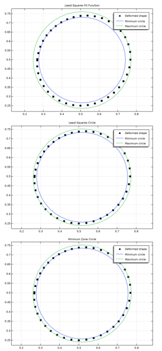
Locate the Data section. From the Dataset list, choose Least-Squares Fit Function/Solution 2 (sol2).
4
Click to expand the Title section. From the Title type list, choose Manual.
5
In the Title text area, type Least-Squares Fit Function.
6
Locate the Axis section. Select the Preserve aspect ratio checkbox.
Deformed Shape
1
Right-click Least-Squares Fit Function and choose Global.
2
In the Settings window for Global, type Deformed Shape in the Label text field.
3
Locate the y-Axis Data section. In the table, enter the following settings:
4
Locate the x-Axis Data section. From the Parameter list, choose Expression.
5
In the Expression text field, type xdata.
6
Click to expand the Coloring and Style section. Find the Line style subsection. From the Line list, choose None.
7
From the Color list, choose Black.
8
Find the Line markers subsection. From the Marker list, choose Point.
9
Click to expand the Legends section. From the Legends list, choose Manual.
10
Minimum Circle
1
In the Model Builder window, right-click Least-Squares Fit Function and choose Global.
2
In the Settings window for Global, type Minimum Circle in the Label text field.
3
Locate the y-Axis Data section. In the table, enter the following settings:
4
Locate the x-Axis Data section. From the Parameter list, choose Expression.
5
In the Expression text field, type x_plot(x_LSQ,Rmin_LSQ).
6
Locate the Legends section. From the Legends list, choose Manual.
7
Maximum Circle
1
Right-click Least-Squares Fit Function and choose Global.
2
In the Settings window for Global, type Maximum Circle in the Label text field.
3
Locate the y-Axis Data section. In the table, enter the following settings:
4
Locate the x-Axis Data section. From the Parameter list, choose Expression.
5
In the Expression text field, type x_plot(x_LSQ,Rmax_LSQ).
6
In the Least-Squares Fit Function toolbar, click  Plot.
7
Locate the Legends section. From the Legends list, choose Manual.
8
Roundness Error
1
In the Results toolbar, click  Evaluation Group.
2
In the Settings window for Evaluation Group, type Roundness Error in the Label text field.
3
Locate the Format section. From the Include parameters list, choose Off.
4
From the Concatenation list, choose Vertical.
LSQ (1)
1
Right-click Roundness Error and choose Global Evaluation.
2
In the Settings window for Global Evaluation, locate the Data section.
3
From the Dataset list, choose Least-Squares Fit Function/Solution 2 (sol2).
4
From the Parameter selection (angle) list, choose Last.
5
Locate the Expressions section. In the table, enter the following settings:
6
In the Label text field, type LSQ (1).
7
In the Roundness Error toolbar, click  Evaluate.
Least Square Circle
Global Definitions
Parameters 1
1
In the Model Builder window, under Global Definitions click Parameters 1.
2
In the Settings window for Parameters, locate the Parameters section.
3
Definitions
Variables 2
1
In the Model Builder window, under Component 1 (comp1) > Definitions click Variables 2.
2
In the Settings window for Variables, locate the Variables section.
3
Add Study
1
In the Home toolbar, click  Add Study to open the Add Study window.
2
Go to the Add Study window.
3
Find the Studies subsection. In the Select Study tree, select General Studies > Stationary.
4
Find the Physics interfaces in study subsection. In the table, clear the Solve checkbox for Solid Mechanics (solid).
5
Find the Studies subsection. In the Select Study tree, select Preset Studies for Selected Physics Interfaces > Stationary.
6
7
In the Home toolbar, click  Add Study to close the Add Study window.
Least-Squares Circle
In the Settings window for Study, type Least-Squares Circle in the Label text field.
Step 1: Stationary
1
In the Model Builder window, under Least-Squares Circle click Step 1: Stationary.
2
In the Settings window for Stationary, locate the Values of Dependent Variables section.
3
Find the Values of variables not solved for subsection. From the Settings list, choose User controlled.
4
From the Method list, choose Solution.
5
From the Study list, choose Study 1, Stationary.
6
From the Parameter value (p (Pa)) list, choose Last.
7
Locate the Study Extensions section. Select the Auxiliary sweep checkbox.
8
Locate the Study Settings section. Select the Include geometric nonlinearity checkbox.
9
Locate the Study Extensions section. Click  Add.
10
General Optimization
1
In the Study toolbar, click  Optimization and choose General Optimization.
2
In the Settings window for General Optimization, locate the Optimization Solver section.
3
From the Method list, choose IPOPT.
4
Locate the Objective Function section. In the table, enter the following settings:
5
Locate the Control Variables and Parameters section. Click  Add three times.
6
7
Locate the Constraints section. In the table, enter the following settings:
8
In the Study toolbar, click  Compute.
Results
Least-Squares Circle
1
In the Model Builder window, right-click Least-Squares Fit Function and choose Duplicate.
2
In the Settings window for 1D Plot Group, type Least-Squares Circle in the Label text field.
3
Locate the Data section. From the Dataset list, choose Least-Squares Circle/Solution 3 (sol3).
4
Locate the Title section. In the Title text area, type Least-Squares Circle.
Minimum Circle
1
In the Model Builder window, expand the Least-Squares Circle node, then click Minimum Circle.
2
In the Settings window for Global, locate the y-Axis Data section.
3
4
Locate the x-Axis Data section. In the Expression text field, type x_plot(x_LSC,Rmin_LSC).
Maximum Circle
1
In the Model Builder window, click Maximum Circle.
2
In the Settings window for Global, locate the y-Axis Data section.
3
4
Locate the x-Axis Data section. In the Expression text field, type x_plot(x_LSC,Rmax_LSC).
5
In the Least-Squares Circle toolbar, click  Plot.
LSC (2)
1
In the Model Builder window, right-click Roundness Error and choose Global Evaluation.
2
In the Settings window for Global Evaluation, type LSC (2) in the Label text field.
3
Locate the Data section. From the Dataset list, choose Least-Squares Circle/Solution 3 (sol3).
4
From the Parameter selection (angle) list, choose Last.
5
Locate the Expressions section. In the table, enter the following settings:
6
In the Roundness Error toolbar, click  Evaluate.
Minimum Zone Circle
Global Definitions
Parameters 1
1
In the Model Builder window, under Global Definitions click Parameters 1.
2
In the Settings window for Parameters, locate the Parameters section.
3
Add Study
1
In the Home toolbar, click  Add Study to open the Add Study window.
2
Go to the Add Study window.
3
Find the Studies subsection. In the Select Study tree, select General Studies > Stationary.
4
Find the Physics interfaces in study subsection. In the table, clear the Solve checkbox for Solid Mechanics (solid).
5
Find the Studies subsection. In the Select Study tree, select Preset Studies for Selected Physics Interfaces > Stationary.
6
7
In the Home toolbar, click  Add Study to close the Add Study window.
Minimum Zone Circle
In the Settings window for Study, type Minimum Zone Circle in the Label text field.
Step 1: Stationary
1
In the Model Builder window, under Minimum Zone Circle click Step 1: Stationary.
2
In the Settings window for Stationary, locate the Values of Dependent Variables section.
3
Find the Values of variables not solved for subsection. From the Settings list, choose User controlled.
4
From the Method list, choose Solution.
5
From the Study list, choose Study 1, Stationary.
6
From the Parameter value (p (Pa)) list, choose Last.
7
Locate the Study Extensions section. Select the Auxiliary sweep checkbox.
8
Locate the Study Settings section. Select the Include geometric nonlinearity checkbox.
9
Locate the Study Extensions section. Click  Add.
10
General Optimization
1
In the Study toolbar, click  Optimization and choose General Optimization.
2
In the Settings window for General Optimization, locate the Optimization Solver section.
3
From the Method list, choose IPOPT.
4
Locate the Objective Function section. In the table, enter the following settings:
5
Locate the Control Variables and Parameters section. Click  Add four times.
6
7
Locate the Constraints section. In the table, enter the following settings:
8
In the Study toolbar, click  Compute.
Results
Minimum Zone Circle
1
In the Model Builder window, right-click Least-Squares Fit Function and choose Duplicate.
2
In the Settings window for 1D Plot Group, type Minimum Zone Circle in the Label text field.
3
Locate the Data section. From the Dataset list, choose Minimum Zone Circle/Solution 4 (sol4).
4
Locate the Title section. In the Title text area, type Minimum Zone Circle.
Minimum Circle
1
In the Model Builder window, expand the Minimum Zone Circle node, then click Minimum Circle.
2
In the Settings window for Global, locate the y-Axis Data section.
3
4
Locate the x-Axis Data section. In the Expression text field, type x_plot(x_MZC,Rmin_MZC).
Maximum Circle
1
In the Model Builder window, click Maximum Circle.
2
In the Settings window for Global, locate the y-Axis Data section.
3
4
Locate the x-Axis Data section. In the Expression text field, type x_plot(x_MZC,Rmax_MZC).
5
In the Minimum Zone Circle toolbar, click  Plot.
MZC (3)
1
In the Model Builder window, right-click Roundness Error and choose Global Evaluation.
2
In the Settings window for Global Evaluation, type MZC (3) in the Label text field.
3
Locate the Data section. From the Dataset list, choose Minimum Zone Circle/Solution 4 (sol4).
4
From the Parameter selection (angle) list, choose Last.
5
Locate the Expressions section. In the table, enter the following settings:
6
In the Roundness Error toolbar, click  Evaluate.
Minimum Circumscribed Circle
Global Definitions
Parameters 1
1
In the Model Builder window, under Global Definitions click Parameters 1.
2
In the Settings window for Parameters, locate the Parameters section.
3
Definitions
Variables 2
1
In the Model Builder window, under Component 1 (comp1) > Definitions click Variables 2.
2
In the Settings window for Variables, locate the Variables section.
3
Add Study
1
In the Home toolbar, click  Add Study to open the Add Study window.
2
Go to the Add Study window.
3
Find the Studies subsection. In the Select Study tree, select General Studies > Stationary.
4
Find the Physics interfaces in study subsection. In the table, clear the Solve checkbox for Solid Mechanics (solid).
5
Find the Studies subsection. In the Select Study tree, select Preset Studies for Selected Physics Interfaces > Stationary.
6
7
In the Home toolbar, click  Add Study to close the Add Study window.
Minimum Circumscribed Circle
In the Settings window for Study, type Minimum Circumscribed Circle in the Label text field.
Step 1: Stationary
1
In the Model Builder window, under Minimum Circumscribed Circle click Step 1: Stationary.
2
In the Settings window for Stationary, locate the Values of Dependent Variables section.
3
Find the Values of variables not solved for subsection. From the Settings list, choose User controlled.
4
From the Method list, choose Solution.
5
From the Study list, choose Study 1, Stationary.
6
From the Parameter value (p (Pa)) list, choose Last.
7
Locate the Study Extensions section. Select the Auxiliary sweep checkbox.
8
Locate the Study Settings section. Select the Include geometric nonlinearity checkbox.
9
Locate the Study Extensions section. Click  Add.
10
General Optimization
1
In the Study toolbar, click  Optimization and choose General Optimization.
2
In the Settings window for General Optimization, locate the Optimization Solver section.
3
From the Method list, choose IPOPT.
4
Locate the Objective Function section. In the table, enter the following settings:
5
Locate the Control Variables and Parameters section. Click  Add three times.
6
7
Locate the Constraints section. In the table, enter the following settings:
8
In the Study toolbar, click  Compute.
Results
Minimum Circumscribed Circle
1
In the Model Builder window, right-click Least-Squares Fit Function and choose Duplicate.
2
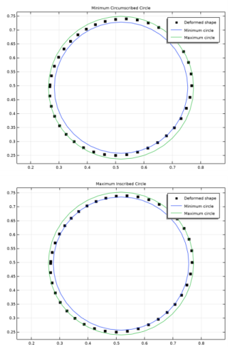
In the Settings window for 1D Plot Group, type Minimum Circumscribed Circle in the Label text field.
3
Locate the Data section. From the Dataset list, choose Minimum Circumscribed Circle/Solution 5 (sol5).
4
Locate the Title section. In the Title text area, type Minimum Circumscribed Circle.
Minimum Circle
1
In the Model Builder window, expand the Minimum Circumscribed Circle node, then click Minimum Circle.
2
In the Settings window for Global, locate the y-Axis Data section.
3
4
Locate the x-Axis Data section. In the Expression text field, type x_plot(x_MCC,Rmin_MCC).
Maximum Circle
1
In the Model Builder window, click Maximum Circle.
2
In the Settings window for Global, locate the y-Axis Data section.
3
4
Locate the x-Axis Data section. In the Expression text field, type x_plot(x_MCC,Rmax_MCC).
5
In the Minimum Circumscribed Circle toolbar, click  Plot.
MCC (4)
1
In the Model Builder window, right-click Roundness Error and choose Global Evaluation.
2
In the Settings window for Global Evaluation, type MCC (4) in the Label text field.
3
Locate the Data section. From the Dataset list, choose Minimum Circumscribed Circle/Solution 5 (sol5).
4
From the Parameter selection (angle) list, choose Last.
5
Locate the Expressions section. In the table, enter the following settings:
6
In the Roundness Error toolbar, click  Evaluate.
Maximum Inscribed Circle
Global Definitions
Parameters 1
1
In the Model Builder window, under Global Definitions click Parameters 1.
2
In the Settings window for Parameters, locate the Parameters section.
3
Definitions
Variables 2
1
In the Model Builder window, under Component 1 (comp1) > Definitions click Variables 2.
2
In the Settings window for Variables, locate the Variables section.
3
Add Study
1
In the Home toolbar, click  Add Study to open the Add Study window.
2
Go to the Add Study window.
3
Find the Studies subsection. In the Select Study tree, select General Studies > Stationary.
4
Find the Physics interfaces in study subsection. In the table, clear the Solve checkbox for Solid Mechanics (solid).
5
Find the Studies subsection. In the Select Study tree, select Preset Studies for Selected Physics Interfaces > Stationary.
6
7
In the Home toolbar, click  Add Study to close the Add Study window.
Maximum Inscribed Circle
In the Settings window for Study, type Maximum Inscribed Circle in the Label text field.
Step 1: Stationary
1
In the Model Builder window, under Maximum Inscribed Circle click Step 1: Stationary.
2
In the Settings window for Stationary, locate the Values of Dependent Variables section.
3
Find the Values of variables not solved for subsection. From the Settings list, choose User controlled.
4
From the Method list, choose Solution.
5
From the Study list, choose Study 1, Stationary.
6
From the Parameter value (p (Pa)) list, choose Last.
7
Locate the Study Extensions section. Select the Auxiliary sweep checkbox.
8
Locate the Study Settings section. Select the Include geometric nonlinearity checkbox.
9
Locate the Study Extensions section. Click  Add.
10
General Optimization
1
In the Study toolbar, click  Optimization and choose General Optimization.
2
In the Settings window for General Optimization, locate the Optimization Solver section.
3
From the Method list, choose IPOPT.
4
Locate the Objective Function section. In the table, enter the following settings:
5
From the Type list, choose Maximization.
6
Locate the Control Variables and Parameters section. Click  Add three times.
7
8
Locate the Constraints section. In the table, enter the following settings:
9
In the Study toolbar, click  Compute.
Results
Maximum Inscribed Circle
1
In the Model Builder window, right-click Least-Squares Fit Function and choose Duplicate.
2
In the Settings window for 1D Plot Group, type Maximum Inscribed Circle in the Label text field.
3
Locate the Data section. From the Dataset list, choose Maximum Inscribed Circle/Solution 6 (sol6).
4
Locate the Title section. In the Title text area, type Maximum Inscribed Circle.
Minimum Circle
1
In the Model Builder window, expand the Maximum Inscribed Circle node, then click Minimum Circle.
2
In the Settings window for Global, locate the y-Axis Data section.
3
4
Locate the x-Axis Data section. In the Expression text field, type x_plot(x_MIC,Rmin_MIC).
Maximum Circle
1
In the Model Builder window, click Maximum Circle.
2
In the Settings window for Global, locate the y-Axis Data section.
3
4
Locate the x-Axis Data section. In the Expression text field, type x_plot(x_MIC,Rmax_MIC).
5
In the Maximum Inscribed Circle toolbar, click  Plot.
MIC (5)
1
In the Model Builder window, right-click Roundness Error and choose Global Evaluation.
2
In the Settings window for Global Evaluation, type MIC (5) in the Label text field.
3
Locate the Data section. From the Dataset list, choose Maximum Inscribed Circle/Solution 6 (sol6).
4
From the Parameter selection (angle) list, choose Last.
5
Locate the Expressions section. In the table, enter the following settings:
6
In the Roundness Error toolbar, click  Evaluate.