PDF

Impact Between Two Soft Rings
Introduction
In this conceptual example, the soft impact between two elastic rings is modeled using the Solid Mechanics interface. The goal is to verify that the contact formulations conserve fundamental thermodynamic quantities such as momentum (linear and angular) and energy. The setup of the problem is based on a benchmark example from Ref. 1.
Model Definition
As illustrated in Figure 1, the 2D geometry consists of two thin rings. Both rings are 30 cm thick and have an outer diameter of 20 m.
Figure 1: Model geometry.
The material of the rings is considered to be linear elastic, with material properties according to Table 1.
The pressure contact is modeled using two different formulations available in COMSOL Multiphysics: Penalty, dynamic and Augmented Lagrangian, dynamic. Both formulations are based on a viscous implementation, where the rate of the gap distance between the source and destination boundaries is constrained to zero once contact is detected. Such formulation assumes that the event dissipates energy, and it is therefore mainly suitable for short impact events.
The uppermost ring is given an initial vertical velocity of -4 m/s to initiate the impact event. No other constraints nor external forces are considered in the model.
Results and Discussion
Figure 2 shows snapshots of the deformed shape of the two rings for every 5 seconds. It can be seen that both rings deform significantly once ring 1 impacts ring 2, and that after the impact the ring 2 gained some of the momentum from ring 1. Also, both rings start to rotate after the impact. It can also be seen that the dynamic penalty method generates a significant overlap between the two geometries during contact. This is expected form the method, since constraints are only added in the step after contact is detected.
Figure 2: Computed deformation of the two rings using the dynamic penalty formulation plotted every 5 seconds.
The impact event can be studied in detail by examining different thermodynamic quantities. Figure 3 and Figure 4 show the linear momentum for each ring and for the total assembly. It can be observed how the initial linear momentum in the y direction of ring 1 is partially transferred to ring 2. During the impact, both rings also gain momentum in the x direction but in opposite directions. Importantly, it can be observed that the linear momentum of the assembly is conserved during the impact event. From Figure 5 it can be seen that both rings also gain angular momentum, which corresponds to the observed rotational movement of the rings. The total angular momentum is also properly conserved.
Figure 6 depicts the energy balance of the assembly and different components of the total energy. Parts of the initial kinetic energy of ring 1 is converted to elastic energy during and after the impact, as both rings deform. Also, the contact between the rings dissipate energy since a viscous formulation is used. The total energy is kept constant throughout the simulation, meaning that the model is consistent in terms of energy.
The conclusions obtained after inspecting the results in Figure 3 to Figure 6 apply to both the dynamic penalty and dynamic augmented Lagrangian formulations. However, the results differ slightly, given that the two formulations enforce the contact constraint in different ways.
Figure 3: Variation of linear momentum in the x direction. Solid lines correspond to the penalty formulation and dashed lines to the augmented Lagrangian formulation.
Figure 4: Variation of linear momentum in the y direction. Solid lines correspond to the penalty formulation and dashed lines to the augmented Lagrangian formulation.
Figure 5: Variation of angular momentum. Solid lines correspond to the penalty formulation and dashed lines to the augmented Lagrangian formulation.
Figure 6: Variation of different energy quantities. Solid lines correspond to the penalty formulation and dashed lines to the augmented Lagrangian formulation.
Notes About the COMSOL Implementation
The two viscous formulations for contact use a penalty factor that is interpreted as an artificial viscosity. Hence, a time scale has to be given as a user input. This characteristic time can be related to the duration of the impact event, or used as a multiplier to find a stable definition of the contact model.
It is often a good practice to use a manual time-step control for this type of dynamic simulation, when the kinematics of the contacting bodies is the main interest. Otherwise, the error estimates used by the automatic time-step control will enforce unnecessary small time steps to resolve the wave propagation within the solid, which is not of primary interest.
Reference
1. T.A. Laursen, Computational Contact and Impact Mechanics: Fundamentals of Modelling Interfacial Phenomena in Nonlinear Finite Element Analysis, Springer-Verlag, 2002.
Application Library path: Structural_Mechanics_Module/Verification_Examples/ring_impact
Modeling Instructions
From the File menu, choose New.
New
In the New window, click  Model Wizard.
Model Wizard
1
In the Model Wizard window, click  2D.
2
In the Select Physics tree, select Structural Mechanics > Solid Mechanics (solid).
3
Click Add.
4
Click  Study.
5
In the Select Study tree, select General Studies > Time Dependent.
6
Global Definitions
Parameters 1
1
In the Model Builder window, under Global Definitions click Parameters 1.
2
In the Settings window for Parameters, locate the Parameters section.
3
Geometry 1
Ring 1
1
In the Geometry toolbar, click  Circle.
2
In the Settings window for Circle, locate the Size and Shape section.
3
In the Radius text field, type radius.
4
Click to expand the Layers section. In the table, enter the following settings:
5
In the Label text field, type Ring 1.
6
Locate the Selections of Resulting Entities section. Select the Resulting objects selection checkbox.
7
From the Color list, choose Color 4.
8
Click  Build All Objects.
Ring 2
1
Right-click Ring 1 and choose Duplicate.
2
In the Settings window for Circle, locate the Position section.
3
In the x text field, type 10.
4
In the y text field, type -20.
5
In the Label text field, type Ring 2.
6
Locate the Selections of Resulting Entities section. From the Color list, choose Color 12.
Delete Entities 1 (del1)
1
In the Model Builder window, right-click Geometry 1 and choose Delete Entities.
2
Click in the Graphics window and then press Ctrl+D to clear all objects.
3
In the Settings window for Delete Entities, locate the Entities or Objects to Delete section.
4
From the Geometric entity level list, choose Domain.
5
On the object c1, select Domain 5 only.
6
On the object c2, select Domain 5 only.
Form Union (fin)
1
In the Model Builder window, click Form Union (fin).
2
In the Settings window for Form Union/Assembly, click  Build Selected.
3
Click the  Zoom Extents button in the Graphics toolbar.
Definitions
Contact Pair 1 (p1)
1
In the Definitions toolbar, click  Pairs and choose Contact Pair.
2
3
In the Settings window for Pair, locate the Destination Boundaries section.
4
Click to select the  Activate Selection toggle button.
5
Materials
Material 1 (mat1)
1
In the Model Builder window, under Component 1 (comp1) right-click Materials and choose Blank Material.
2
In the Settings window for Material, locate the Material Contents section.
3
Solid Mechanics (solid)
Initial Values 2
1
In the Physics toolbar, click  Domains and choose Initial Values.
2
In the Settings window for Initial Values, locate the Domain Selection section.
3
From the Selection list, choose Ring 1.
4
Contact 1
1
In the Model Builder window, click Contact 1.
2
In the Settings window for Contact, locate the Contact Method section.
3
From the list, choose Penalty, dynamic.
For impact problems, a purely viscous penalty formulation is preferable.
4
Locate the Contact Pressure Penalty Factor section. From the Penalty factor control list, choose Viscous only.
5
In the τn text field, type .1[ms].
Enable Advanced Physics Options to compute energy dissipation.
6
Click the  Show More Options button in the Model Builder toolbar.
7
In the Show More Options dialog, in the tree, select the checkbox for the node Physics > Advanced Physics Options.
8
9
In the Settings window for Contact, click to expand the Advanced section.
10
Select the Compute viscous contact dissipation checkbox.
Also, solve the model using the dynamic augmented Lagrangian formulation.
Contact 2
1
Right-click Component 1 (comp1) > Solid Mechanics (solid) > Contact 1 and choose Duplicate.
2
In the Settings window for Contact, locate the Pair Selection section.
3
From the Pairs list, choose From list.
4
5
In the Add dialog, select Contact Pair 1 (p1) in the Pairs list.
6
7
In the Settings window for Contact, locate the Contact Method section.
8
From the list, choose Augmented Lagrangian, dynamic.
9
Locate the Contact Pressure Penalty Factor section. In the τn text field, type .01[ms].
Mesh 1
Mapped 1
In the Mesh toolbar, click  Mapped.
Distribution 1
1
Right-click Mapped 1 and choose Distribution.
2
3
In the Settings window for Distribution, locate the Distribution section.
4
In the Number of elements text field, type 3.
Distribution 2
1
In the Model Builder window, right-click Mapped 1 and choose Distribution.
2
3
In the Settings window for Distribution, locate the Distribution section.
4
In the Number of elements text field, type 20.
5
Click  Build All.
Study 1: Penalty
Use the dynamic penalty formulation in the first study.
1
In the Model Builder window, click Study 1.
2
In the Settings window for Study, type Study 1: Penalty in the Label text field.
Step 1: Time Dependent
1
In the Model Builder window, under Study 1: Penalty click Step 1: Time Dependent.
2
In the Settings window for Time Dependent, locate the Study Settings section.
3
In the Output times text field, type range(0,0.1,20).
4
Locate the Physics and Variables Selection section. Select the Modify model configuration for study step checkbox.
5
In the tree, select Component 1 (comp1) > Solid Mechanics (solid), Controls spatial frame > Contact 2.
6
Modify the time-dependent solver to use a manual time step control.
Solution 1 (sol1)
1
In the Study toolbar, click  Show Default Solver.
2
In the Model Builder window, expand the Solution 1 (sol1) node, then click Time-Dependent Solver 1.
3
In the Settings window for Time-Dependent Solver, click to expand the Time Stepping section.
4
From the Steps taken by solver list, choose Manual.
5
In the Time step text field, type 0.05.
6
In the Study toolbar, click  Compute.
Results
Deformation (Penalty)
In the Settings window for 2D Plot Group, type Deformation (Penalty) in the Label text field.
Surface 1
1
In the Model Builder window, expand the Deformation (Penalty) node, then click Surface 1.
2
In the Settings window for Surface, locate the Expression section.
3
In the Expression text field, type 1.
4
Click to expand the Title section. From the Title type list, choose None.
5
Locate the Coloring and Style section. From the Coloring list, choose Uniform.
6
From the Color list, choose Yellow.
Selection 1
1
Right-click Surface 1 and choose Selection.
2
In the Settings window for Selection, locate the Selection section.
3
From the Selection list, choose Ring 1.
Surface 2
1
Right-click Surface 1 and choose Duplicate.
2
In the Settings window for Surface, locate the Coloring and Style section.
3
From the Color list, choose Red.
Selection 1
1
In the Model Builder window, expand the Surface 2 node, then click Selection 1.
2
In the Settings window for Selection, locate the Selection section.
3
From the Selection list, choose Ring 2.
4
In the Deformation (Penalty) toolbar, click  Plot.
5
Click the  Zoom Extents button in the Graphics toolbar.
Deformation (Penalty)
In the Model Builder window, under Results click Deformation (Penalty).
Animation 1
1
In the Deformation (Penalty) toolbar, click  Animation and choose Player.
2
In the Settings window for Animation, locate the Frames section.
3
In the Number of frames text field, type 100.
4
Click the  Zoom Extents button in the Graphics toolbar.
5
Click the  Play button in the Graphics toolbar.
Add Study
Create a second study for the dynamic augmented Lagrangian formulation.
1
In the Home toolbar, click  Add Study to open the Add Study window.
2
Go to the Add Study window.
3
Find the Studies subsection. In the Select Study tree, select General Studies > Time Dependent.
4
Click the Add Study button in the window toolbar.
5
In the Home toolbar, click  Add Study to close the Add Study window.
Study 2: Augmented Lagrangian
In the Settings window for Study, type Study 2: Augmented Lagrangian in the Label text field.
Step 1: Time Dependent
1
In the Model Builder window, under Study 2: Augmented Lagrangian click Step 1: Time Dependent.
2
In the Settings window for Time Dependent, locate the Study Settings section.
3
In the Output times text field, type range(0,0.1,20).
Solution 2 (sol2)
1
In the Study toolbar, click  Show Default Solver.
2
In the Model Builder window, expand the Solution 2 (sol2) node, then click Time-Dependent Solver 1.
3
In the Settings window for Time-Dependent Solver, locate the Time Stepping section.
4
From the Steps taken by solver list, choose Manual.
5
In the Time step text field, type 0.05.
Increase the number of iterations allowed for the segregated solver.
6
In the Model Builder window, expand the Study 2: Augmented Lagrangian > Solver Configurations > Solution 2 (sol2) > Time-Dependent Solver 1 node, then click Segregated 1.
7
In the Settings window for Segregated, locate the General section.
8
In the Maximum number of iterations text field, type 50.
9
In the Study toolbar, click  Compute.
Results
Deformation (AugLag)
In the Settings window for 2D Plot Group, type Deformation (AugLag) in the Label text field.
Surface 1
1
In the Model Builder window, expand the Deformation (AugLag) node, then click Surface 1.
2
In the Settings window for Surface, locate the Expression section.
3
In the Expression text field, type 1.
4
Locate the Title section. From the Title type list, choose None.
5
Locate the Coloring and Style section. From the Coloring list, choose Uniform.
6
From the Color list, choose Yellow.
Selection 1
1
Right-click Surface 1 and choose Selection.
2
In the Settings window for Selection, locate the Selection section.
3
From the Selection list, choose Ring 1.
Surface 2
1
Right-click Surface 1 and choose Duplicate.
2
In the Settings window for Surface, locate the Coloring and Style section.
3
From the Color list, choose Red.
Selection 1
1
In the Model Builder window, expand the Surface 2 node, then click Selection 1.
2
In the Settings window for Selection, locate the Selection section.
3
From the Selection list, choose Ring 2.
4
In the Deformation (AugLag) toolbar, click  Plot.
5
Click the  Zoom Extents button in the Graphics toolbar.
Deformation (AugLag)
In the Model Builder window, under Results click Deformation (AugLag).
Animation 2
1
In the Deformation (AugLag) toolbar, click  Animation and choose Player.
2
Click the  Zoom Extents button in the Graphics toolbar.
3
In the Settings window for Animation, locate the Frames section.
4
In the Number of frames text field, type 100.
5
Click the  Play button in the Graphics toolbar.
Energy Balance
1
In the Results toolbar, click  1D Plot Group.
2
In the Settings window for 1D Plot Group, type Energy Balance in the Label text field.
3
Click to expand the Title section. From the Title type list, choose Label.
Global 1
1
Right-click Energy Balance and choose Global.
2
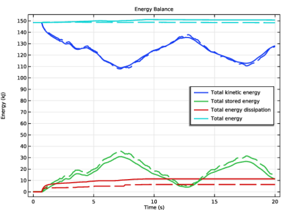
In the Settings window for Global, click Replace Expression in the upper-right corner of the y-Axis Data section. From the menu, choose Component 1 (comp1) > Solid Mechanics > Global > solid.Wk_tot - Total kinetic energy - J.
3
Click Add Expression in the upper-right corner of the y-Axis Data section. From the menu, choose Component 1 (comp1) > Solid Mechanics > Global > solid.Wh_tot - Total stored energy - J.
4
Click Add Expression in the upper-right corner of the y-Axis Data section. From the menu, choose Component 1 (comp1) > Solid Mechanics > Global > solid.Wd_tot - Total energy dissipation - J.
5
In the Energy Balance toolbar, click  Plot.
6
Locate the y-Axis Data section. In the table, enter the following settings:
7
Click to expand the Coloring and Style section. From the Width list, choose 2.
Plot the energy balance for the dynamic augmented Lagrangian formulation using dashed lines.
Global 2
1
Right-click Global 1 and choose Duplicate.
2
In the Settings window for Global, locate the Data section.
3
From the Dataset list, choose Study 2: Augmented Lagrangian/Solution 2 (sol2).
4
Locate the Coloring and Style section. Find the Line style subsection. From the Line list, choose Dashed.
5
From the Color list, choose Cycle (reset).
6
Click to expand the Legends section. Clear the Show legends checkbox.
Energy Balance
1
In the Model Builder window, click Energy Balance.
2
In the Settings window for 1D Plot Group, locate the Plot Settings section.
3
Select the y-axis label checkbox. In the associated text field, type Energy (kJ).
4
Locate the Legend section. From the Position list, choose Middle right.
5
In the Energy Balance toolbar, click  Plot.
Create evaluation groups to compute the linear and angular momentum of the rings.
Linear Momentum, x (Penalty)
1
In the Results toolbar, click  Evaluation Group.
2
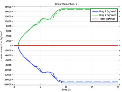
In the Settings window for Evaluation Group, type Linear Momentum, x (Penalty) in the Label text field.
Surface Integration 1
1
Right-click Linear Momentum, x (Penalty) and choose Integration > Surface Integration.
2
In the Settings window for Surface Integration, locate the Selection section.
3
From the Selection list, choose Ring 1.
4
Locate the Expressions section. In the table, enter the following settings:
Surface Integration 2
1
Right-click Surface Integration 1 and choose Duplicate.
2
In the Settings window for Surface Integration, locate the Selection section.
3
From the Selection list, choose Ring 2.
4
Locate the Expressions section. In the table, enter the following settings:
Surface Integration 3
1
Right-click Surface Integration 2 and choose Duplicate.
2
In the Settings window for Surface Integration, locate the Selection section.
3
From the Selection list, choose All domains.
4
Locate the Expressions section. In the table, enter the following settings:
5
In the Linear Momentum, x (Penalty) toolbar, click  Evaluate.
Linear Momentum, x (AugLag)
1
In the Model Builder window, right-click Linear Momentum, x (Penalty) and choose Duplicate.
2
In the Settings window for Evaluation Group, type Linear Momentum, x (AugLag) in the Label text field.
3
Locate the Data section. From the Dataset list, choose Study 2: Augmented Lagrangian/Solution 2 (sol2).
4
In the Linear Momentum, x (AugLag) toolbar, click  Evaluate.
Linear Momentum, y (Penalty)
1
Right-click Linear Momentum, x (Penalty) and choose Duplicate.
2
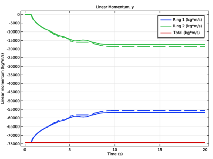
In the Settings window for Evaluation Group, type Linear Momentum, y (Penalty) in the Label text field.
Surface Integration 1
1
In the Model Builder window, expand the Linear Momentum, y  (Penalty) node, then click Surface Integration 1.
2
In the Settings window for Surface Integration, locate the Expressions section.
3
Surface Integration 2
1
In the Model Builder window, click Surface Integration 2.
2
In the Settings window for Surface Integration, locate the Expressions section.
3
Surface Integration 3
1
In the Model Builder window, click Surface Integration 3.
2
In the Settings window for Surface Integration, locate the Expressions section.
3
4
In the Linear Momentum, y (Penalty) toolbar, click  Evaluate.
Linear Momentum, y (AugLag)
1
In the Model Builder window, right-click Linear Momentum, y  (Penalty) and choose Duplicate.
2
In the Settings window for Evaluation Group, type Linear Momentum, y (AugLag) in the Label text field.
3
Locate the Data section. From the Dataset list, choose Study 2: Augmented Lagrangian/Solution 2 (sol2).
4
In the Linear Momentum, y (AugLag) toolbar, click  Evaluate.
Angular Momentum (Penalty)
1
In the Model Builder window, right-click Linear Momentum, x (Penalty) and choose Duplicate.
2
In the Model Builder window, click Linear Momentum, x (Penalty) 1.
3
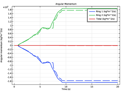
In the Settings window for Evaluation Group, type Angular Momentum (Penalty) in the Label text field.
Surface Integration 1
1
In the Model Builder window, click Surface Integration 1.
2
In the Settings window for Surface Integration, locate the Expressions section.
3
Surface Integration 2
1
In the Model Builder window, click Surface Integration 2.
2
In the Settings window for Surface Integration, locate the Expressions section.
3
Surface Integration 3
1
In the Model Builder window, click Surface Integration 3.
2
In the Settings window for Surface Integration, locate the Expressions section.
3
4
In the Angular Momentum (Penalty) toolbar, click  Evaluate.
Angular Momentum (AugLag)
1
In the Model Builder window, right-click Angular Momentum (Penalty) and choose Duplicate.
2
In the Settings window for Evaluation Group, type Angular Momentum (AugLag) in the Label text field.
3
Locate the Data section. From the Dataset list, choose Study 2: Augmented Lagrangian/Solution 2 (sol2).
4
In the Angular Momentum (AugLag) toolbar, click  Evaluate.
Linear Momentum, x
1
In the Results toolbar, click  1D Plot Group.
2
In the Settings window for 1D Plot Group, type Linear Momentum, x in the Label text field.
3
Locate the Title section. From the Title type list, choose Label.
4
Locate the Plot Settings section.
5
Select the y-axis label checkbox. In the associated text field, type Linear momentum (kg*m/s).
Table Graph 1
1
Right-click Linear Momentum, x and choose Table Graph.
2
In the Settings window for Table Graph, locate the Data section.
3
From the Source list, choose Evaluation group.
4
Locate the Coloring and Style section. From the Width list, choose 2.
5
Click to expand the Legends section. Select the Show legends checkbox.
Table Graph 2
1
Right-click Table Graph 1 and choose Duplicate.
2
In the Settings window for Table Graph, locate the Data section.
3
From the Evaluation group list, choose Linear Momentum, x (AugLag).
4
Locate the Coloring and Style section. Find the Line style subsection. From the Line list, choose Dashed.
5
From the Color list, choose Cycle (reset).
6
Locate the Legends section. Clear the Show legends checkbox.
7
In the Linear Momentum, x toolbar, click  Plot.
Linear Momentum, y
1
In the Model Builder window, right-click Linear Momentum, x and choose Duplicate.
2
In the Settings window for 1D Plot Group, type Linear Momentum, y in the Label text field.
Table Graph 1
1
In the Model Builder window, expand the Linear Momentum, y node, then click Table Graph 1.
2
In the Settings window for Table Graph, locate the Data section.
3
From the Evaluation group list, choose Linear Momentum, y  (Penalty).
Table Graph 2
1
In the Model Builder window, click Table Graph 2.
2
In the Settings window for Table Graph, locate the Data section.
3
From the Evaluation group list, choose Linear Momentum, y (AugLag).
4
In the Linear Momentum, y toolbar, click  Plot.
Angular Momentum
1
In the Model Builder window, right-click Linear Momentum, y and choose Duplicate.
2
In the Settings window for 1D Plot Group, type Angular Momentum in the Label text field.
3
Locate the Plot Settings section. In the y-axis label text field, type Angular momentum (kg*m^2/s).
Table Graph 1
1
In the Model Builder window, expand the Angular Momentum node, then click Table Graph 1.
2
In the Settings window for Table Graph, locate the Data section.
3
From the Evaluation group list, choose Angular Momentum (Penalty).
Table Graph 2
1
In the Model Builder window, click Table Graph 2.
2
In the Settings window for Table Graph, locate the Data section.
3
From the Evaluation group list, choose Angular Momentum (AugLag).
4
In the Angular Momentum toolbar, click  Plot.