PDF

Submodel in a Wheel Rim
Introduction
In stress analysis, it is common that the regions with high stresses are small when compared to the whole structure. Sometimes it is not feasible to have a mesh that at the same time captures the global behavior and resolves the stress concentrations with high accuracy. This is especially true in nonlinear or dynamic problems.
You can cope with these types of problems with a technique known as submodeling. First you solve the complete model with a mesh which is sufficient to capture the stiffness of the structure. In a second analysis you create a local model (submodel) of the region around the stress concentration with a fine mesh, and solve it using the displacements from the global model as boundary conditions.
There are some underlying assumptions when using submodels:
This example shows how to perform submodel analysis in COMSOL Multiphysics.
Model Definition
The wheel rim for this analysis has a ten-spoke design, such that the elements of the geometry cause the finite element mesh to become quite large. The loading on the tire is composed of both the tire pressure and a load transferred from the road via the tire to the rim.
In the submodel (shown in Figure 1), you cut out a small region around the hotspot using an intersection between the rim geometry and a 70 mm-by-70 mm-by-60 mm block.
Figure 1: The submodel geometry.
Material
Aluminum with 70 GPa, ν = 0.33.
Constraints
Loads
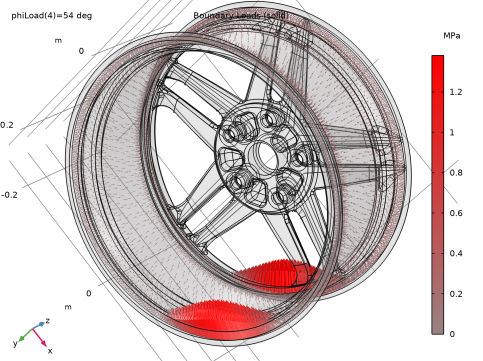
The total load carried by the wheel corresponds to a weight of 1120 kg. It is applied as a pressure on the rim surfaces where the tire is in contact. Assume that the load distribution in the circumferential direction can be approximated as p = p0cos( 3ϑ ), where ϑ is the angle from the point of contact between the road and the tire. The loaded area thus extends 30° in each direction from the peak of the load. Four different load cases are analyzed, where the center of the peak load is rotated 18° each time. In this way the whole load cycle for the rotating wheel can be covered. The pressure load and the load distribution carried by the wheel are shown in Figure 2.
Figure 2: Pressure and tire load when rotated 54° from the center of the first pair of spokes.
Results and Discussion
The highest stresses occur in the fillet where the spoke connects to the hub. In the global model the maximum equivalent stress is mesh dependent, and not reliable. In the submodel, where the resolution is good, the von Mises stress is about 98 MPa. It occurs when the load is rotated 18° from the reference angle. In a fatigue analysis, where the lifetime could vary as the fifth power of the stress, it is essential to get this level of accuracy in the critical regions.
Figure 3: Stresses in the global model.
Figure 4: Stresses in the submodel at the load position giving the peak von Mises stress.
Notes About the COMSOL Implementation
Two different components are used within the same MPH file. In the global model, a general extrusion feature is introduced in order to describe the mapping of results from the global model to the submodel. The general extrusion is parameterized so that displacements from different spokes can be applied to the submodel.
Application Library path: Structural_Mechanics_Module/Tutorials/rim_submodel
Modeling Instructions
From the File menu, choose New.
New
In the New window, click  Model Wizard.
Model Wizard
1
In the Model Wizard window, click  3D.
2
In the Select Physics tree, select Structural Mechanics > Solid Mechanics (solid).
3
Click Add.
4
Click  Study.
5
In the Select Study tree, select General Studies > Stationary.
6
Global Definitions
Parameters 1
1
In the Model Builder window, under Global Definitions click Parameters 1.
2
In the Settings window for Parameters, locate the Parameters section.
3
Geometry 1
1
In the Geometry toolbar, click Insert Sequence and choose Insert Sequence.
2
Import 1 (imp1)
1
In the Model Builder window, under Component 1 (comp1) > Geometry 1 click Import 1 (imp1).
2
In the Settings window for Import, click  Build Selected.
3
Click the  Zoom Extents button in the Graphics toolbar.
Create selections to help with the physics setup. When building the Rotate 1 node, the selections will propagate to the full geometry.
Fixed to Hub
1
In the Geometry toolbar, click  Selections and choose Explicit Selection.
2
In the Settings window for Explicit Selection, type Fixed to Hub in the Label text field.
3
Locate the Entities to Select section. From the Geometric entity level list, choose Boundary.
4
On the object imp1, select Boundaries 10 and 137 only.
Tire Attachment
1
In the Geometry toolbar, click  Selections and choose Explicit Selection.
2
In the Settings window for Explicit Selection, type Tire Attachment in the Label text field.
3
Locate the Entities to Select section. From the Geometric entity level list, choose Boundary.
4
On the object imp1, select Boundaries 47–50 only.
Pressure Surface
1
In the Geometry toolbar, click  Selections and choose Explicit Selection.
2
In the Settings window for Explicit Selection, type Pressure Surface in the Label text field.
3
Locate the Entities to Select section. From the Geometric entity level list, choose Boundary.
4
On the object imp1, select Boundaries 36–38, 41, 42, and 45–50 only.
Fixed to Hub (sel1), Pressure Surface (sel3), Tire Attachment (sel2)
1
In the Model Builder window, under Component 1 (comp1) > Geometry 1, Ctrl-click to select Fixed to Hub (sel1), Tire Attachment (sel2), and Pressure Surface (sel3).
2
Selections
In the Settings window for Group, type Selections in the Label text field.
Remove Details 1 (rmd1)
1
In the Model Builder window, click Remove Details 1 (rmd1).
2
In the Settings window for Remove Details, click  Build Selected.
Add Material
1
In the Materials toolbar, click  Add Material to open the Add Material window.
2
Go to the Add Material window.
3
In the tree, select Built-in > Aluminum.
4
Click the Add to Component button in the window toolbar.
5
In the Materials toolbar, click  Add Material to close the Add Material window.
Materials
Aluminum (mat1)
1
Click the  Show More Options button in the Model Builder toolbar.
2
In the Show More Options dialog, in the tree, select the checkbox for the node Physics > Equation Contributions.
3
Add Material from Library
In the Home toolbar, click  Windows and choose Add Material from Library.
Add Material
1
Go to the Add Material window.
2
In the tree, select Built-in > Structural steel.
3
Click the Add to Component button in the window toolbar.
Materials
Structural steel (mat2)
1
In the Settings window for Material, locate the Geometric Entity Selection section.
2
From the Geometric entity level list, choose Boundary.
3
From the Selection list, choose Fixed to Hub.
Solid Mechanics (solid)
Spring Foundation 1
1
In the Physics toolbar, click  Boundaries and choose Spring Foundation.
2
In the Settings window for Spring Foundation, locate the Boundary Selection section.
3
From the Selection list, choose Fixed to Hub.
4
Locate the Spring section. From the Spring type list, choose Use material data.
5
In the ds text field, type 0.01.
Boundary Load 1
1
In the Physics toolbar, click  Boundaries and choose Boundary Load.
2
In the Settings window for Boundary Load, locate the Boundary Selection section.
3
From the Selection list, choose Pressure Surface.
4
Locate the Force section. From the Load type list, choose Pressure.
5
In the p text field, type pInflation.
Definitions
Analytic 1 (an1)
1
In the Definitions toolbar, click  Analytic.
2
In the Settings window for Analytic, locate the Definition section.
3
In the Expression text field, type (abs(atan2(x,y)-phi)<pi/6)*cos(3*(atan2(x,y)-phi)).
4
In the Arguments text field, type x, y, phi.
5
Locate the Units section. In the table, enter the following settings:
6
In the Function text field, type Pa.
7
In the Function name text field, type loadDistr.
Cylindrical System 2 (sys2)
In the Definitions toolbar, click  Coordinate Systems and choose Cylindrical System.
Solid Mechanics (solid)
Boundary Load 2
1
In the Physics toolbar, click  Boundaries and choose Boundary Load.
2
In the Settings window for Boundary Load, locate the Coordinate System Selection section.
3
From the Coordinate system list, choose Cylindrical System 2 (sys2).
4
Locate the Boundary Selection section. From the Selection list, choose Tire Attachment.
5
Locate the Force section. Specify the fA vector as
Definitions
Integration 1 (intop1)
1
In the Definitions toolbar, click  Nonlocal Couplings and choose Integration.
2
In the Settings window for Integration, locate the Source Selection section.
3
From the Geometric entity level list, choose Boundary.
4
From the Selection list, choose Tire Attachment.
Variables 1
1
In the Model Builder window, right-click Definitions and choose Variables.
2
In the Settings window for Variables, locate the Variables section.
3
Mesh 1
1
In the Model Builder window, under Component 1 (comp1) click Mesh 1.
2
In the Settings window for Mesh, locate the Physics-Controlled Mesh section.
3
From the Element size list, choose Coarser.
4
Click  Build All.
Study 1
Step 1: Stationary
1
In the Model Builder window, under Study 1 click Step 1: Stationary.
2
In the Settings window for Stationary, click to expand the Study Extensions section.
3
Select the Auxiliary sweep checkbox.
4
5
Solution 1 (sol1)
1
In the Study toolbar, click  Show Default Solver.
2
In the Model Builder window, expand the Solution 1 (sol1) node.
Because of the model’s considerable size, you use an iterative solver that can significantly save on the memory needed for the computations. Use the default GMRES iterative solver with Geometric Multigrid as a preconditioner. On the coarse multigrid level, the solver will lower the order in the discretization of the displacement variables from the default quadratic elements to linear elements.
3
In the Model Builder window, expand the Study 1 > Solver Configurations > Solution 1 (sol1) > Stationary Solver 1 node.
4
Right-click Study 1 > Solver Configurations > Solution 1 (sol1) > Stationary Solver 1 > Suggested Iterative Solver (solid) and choose Enable.
5
In the Study toolbar, click  Compute.
Set default units for result presentation.
Results
Preferred Units 1
1
In the Results toolbar, click  Configurations and choose Preferred Units.
2
In the Settings window for Preferred Units, locate the Units section.
3
Click  Add Physical Quantity.
4
In the Physical Quantity dialog, select Solid Mechanics > Stress tensor (N/m^2) in the tree.
5
6
In the Settings window for Preferred Units, locate the Units section.
7
8
Select the Apply conversions to expressions with the same dimensions checkbox.
9
Click  Apply.
Stress (solid)
1
In the Model Builder window, expand the Results > Stress (solid) node, then click Stress (solid).
2
In the Settings window for 3D Plot Group, locate the Data section.
3
From the Parameter value (phiLoad (deg)) list, choose 0.
4
Locate the Plot Settings section. Clear the Plot dataset edges checkbox.
Volume 1
1
In the Model Builder window, click Volume 1.
2
In the Settings window for Volume, click to expand the Range section.
3
Select the Manual color range checkbox.
4
In the Maximum text field, type 90.
To get a better view of the region with the highest stresses (compare with Figure 3), use a View feature node.
Definitions
View 2
1
In the Model Builder window, under Component 1 (comp1) right-click Definitions and choose View.
In the Graphics window, rotate the model and capture the highest stressed part.
2
In the Settings window for View, locate the View section.
3
Select the Lock camera checkbox.
Results
Stress (solid)
1
In the Model Builder window, under Results click Stress (solid).
2
In the Settings window for 3D Plot Group, locate the Plot Settings section.
3
From the View list, choose View 2.
4
In the Stress (solid) toolbar, click  Plot.
Insert a plot showing boundary loads from Result Templates. Change its setting slightly to reproduce Figure 2.
Result Templates
1
In the Results toolbar, click  Result Templates to open the Result Templates window.
2
Go to the Result Templates window.
3
In the tree, select Study 1/Solution 1 (sol1) > Solid Mechanics > Applied Loads (solid) > Boundary Loads (solid).
4
Click the Add Result Template button in the window toolbar.
5
In the Results toolbar, click  Result Templates to close the Result Templates window.
Results
Boundary Load 1
1
In the Model Builder window, expand the Boundary Loads (solid) node, then click Boundary Load 1.
2
In the Settings window for Arrow Surface, locate the Coloring and Style section.
3
Select the Scale factor checkbox. In the associated text field, type 4E-2.
4
In the Boundary Loads (solid) toolbar, click  Plot.
Root
Start creating the submodel.
Add Component
In the Model Builder window, right-click the root node and choose Add Component > 3D.
Geometry 2
Import 1 (imp1)
1
In the Geometry toolbar, click  Import.
2
In the Settings window for Import, locate the Source section.
3
From the Source list, choose Any importable file.
4
Click  Browse.
5
6
Click  Import.
7
Click the  Go to Default View button in the Graphics toolbar.
Prescribed Displacement
1
In the Geometry toolbar, click  Block.
2
In the Settings window for Block, type Prescribed Displacement in the Label text field.
3
Locate the Size and Shape section. In the Width text field, type 6e-2.
4
In the Depth text field, type 7e-2.
5
In the Height text field, type 6e-2.
6
Locate the Position section. In the y text field, type 6.5e-2.
7
In the z text field, type 6e-2.
8
Locate the Selections of Resulting Entities section. Select the Resulting objects selection checkbox.
9
From the Show in physics list, choose Boundary selection.
Intersection 1 (int1)
1
In the Geometry toolbar, click  Booleans and Partitions and choose Intersection.
2
Click in the Graphics window and then press Ctrl+A to select both objects.
3
In the Settings window for Intersection, click  Build Selected.
4
Click the  Zoom Extents button in the Graphics toolbar.
Fixed to Hub
1
In the Geometry toolbar, click  Selections and choose Explicit Selection.
2
In the Settings window for Explicit Selection, type Fixed to Hub in the Label text field.
3
Locate the Entities to Select section. From the Geometric entity level list, choose Boundary.
4
On the object int1, select Boundary 5 only.
5
Click  Build Selected.
Finer Size Setting
1
In the Geometry toolbar, click  Selections and choose Explicit Selection.
2
In the Settings window for Explicit Selection, locate the Entities to Select section.
3
From the Geometric entity level list, choose Boundary.
4
On the object int1, select Boundary 14 only.
5
In the Label text field, type Finer Size Setting.
6
Click  Build Selected.
Finer Size Setting (sel2), Fixed to Hub (sel1)
1
In the Model Builder window, under Component 2 (comp2) > Geometry 2, Ctrl-click to select Fixed to Hub (sel1) and Finer Size Setting (sel2).
2
Selections
In the Settings window for Group, type Selections in the Label text field.
Add Material from Library
In the Home toolbar, click  Windows and choose Add Material from Library.
Add Material
1
Go to the Add Material window.
2
In the tree, select Built-in > Aluminum.
3
Click the Add to Component button in the window toolbar.
4
In the tree, select Built-in > Structural steel.
5
Click the Add to Component button in the window toolbar.
Materials
Structural steel (mat4)
1
In the Settings window for Material, locate the Geometric Entity Selection section.
2
From the Geometric entity level list, choose Boundary.
3
From the Selection list, choose Fixed to Hub.
Definitions (comp1)
In the Model Builder window, under Component 1 (comp1) click Definitions.
General Extrusion 1 (genext1)
1
In the Definitions toolbar, click  Nonlocal Couplings and choose General Extrusion.
2
In the Settings window for General Extrusion, type from_global in the Operator name text field.
3
Locate the Source Selection section. From the Selection list, choose All domains.
4
Locate the Source section. From the Source frame list, choose Material  (X, Y, Z).
5
Locate the Destination Map section. In the X-expression text field, type X*cos(spokeAngle)-Y*sin(spokeAngle).
6
In the Y-expression text field, type Y*cos(spokeAngle)+X*sin(spokeAngle).
7
In the Z-expression text field, type Z.
8
Click to expand the Advanced section. In the Extrapolation tolerance text field, type 0.5.
Component 2 (comp2)
In the Model Builder window, click Component 2 (comp2).
Add Physics
1
In the Home toolbar, click  Add Physics to open the Add Physics window.
2
Go to the Add Physics window.
3
In the tree, select Structural Mechanics > Solid Mechanics (solid).
4
Click the Add to Component 2 button in the window toolbar.
5
In the Home toolbar, click  Add Physics to close the Add Physics window.
Solid Mechanics 2 (solid2)
Spring Foundation 1
1
In the Physics toolbar, click  Boundaries and choose Spring Foundation.
2
In the Settings window for Spring Foundation, locate the Boundary Selection section.
3
From the Selection list, choose Fixed to Hub.
4
Locate the Spring section. From the Spring type list, choose Use material data.
5
In the ds text field, type 0.01.
Prescribed Displacement 1
1
In the Physics toolbar, click  Boundaries and choose Prescribed Displacement.
2
In the Settings window for Prescribed Displacement, locate the Boundary Selection section.
3
From the Selection list, choose Prescribed Displacement.
4
Locate the Prescribed Displacement section. From the Displacement in x direction list, choose Prescribed.
5
In the u0x text field, type comp1.from_global(comp1.u*cos(spokeAngle)+comp1.v*sin(spokeAngle)).
6
From the Displacement in y direction list, choose Prescribed.
7
In the u0y text field, type comp1.from_global(comp1.v*cos(spokeAngle)-comp1.u*sin(spokeAngle)).
8
From the Displacement in z direction list, choose Prescribed.
9
In the u0z text field, type comp1.from_global(comp1.w).
Mesh 2
1
In the Model Builder window, under Component 2 (comp2) click Mesh 2.
2
In the Settings window for Mesh, locate the Physics-Controlled Mesh section.
3
From the Element size list, choose Fine.
4
Locate the Sequence Type section. From the list, choose User-controlled mesh.
Size 1
1
In the Model Builder window, right-click Free Tetrahedral 1 and choose Size.
2
In the Settings window for Size, locate the Geometric Entity Selection section.
3
From the Geometric entity level list, choose Boundary.
4
From the Selection list, choose Finer Size Setting.
5
Locate the Element Size section. From the Predefined list, choose Extremely fine.
6
Click  Build All.
Add Study
1
In the Home toolbar, click  Add Study to open the Add Study window.
2
Go to the Add Study window.
3
Find the Studies subsection. In the Select Study tree, select General Studies > Stationary.
4
Find the Physics interfaces in study subsection. In the table, clear the Solve checkbox for Solid Mechanics (solid).
5
Click the Add Study button in the window toolbar.
6
In the Home toolbar, click  Add Study to close the Add Study window.
Study 2
Step 1: Stationary
1
In the Settings window for Stationary, click to expand the Values of Dependent Variables section.
Fetch the displacements from the solution of the global model.
2
Find the Values of variables not solved for subsection. From the Settings list, choose User controlled.
3
From the Method list, choose Solution.
4
From the Study list, choose Study 1, Stationary.
5
From the Parameter value (phiLoad (deg)) list, choose Automatic (all solutions).
6
Locate the Study Extensions section. Select the Auxiliary sweep checkbox.
7
From the Sweep type list, choose All combinations.
8
9
10
11
Avoid saving a lot of duplicate results for the full geometry.
12
Click to expand the Store in Output section. In the table, enter the following settings:
Solution 2 (sol2)
In the Study toolbar, click  Show Default Solver.
Solution 2 (sol2)
1
In the Model Builder window, expand the Study 2 > Solver Configurations > Solution 2 (sol2) node.
For the submodel, you also use the default suggested iterative solver.
2
In the Model Builder window, expand the Study 2 > Solver Configurations > Solution 2 (sol2) > Stationary Solver 1 node.
3
Right-click Study 2 > Solver Configurations > Solution 2 (sol2) > Stationary Solver 1 > Suggested Iterative Solver (solid2) and choose Enable.
Study 1
Solution 1 (sol1)
In the Model Builder window, expand the Study 2 > Solver Configurations > Solution 2 (sol2) > Stationary Solver 1 > Suggested Iterative Solver (solid2) node.
Study 2
Solution 2 (sol2)
1
In the Model Builder window, expand the Study 1 > Solver Configurations > Solution 1 (sol1) > Stationary Solver 1 > Suggested Iterative Solver (solid) node, then click Study 2 > Solver Configurations > Solution 2 (sol2) > Stationary Solver 1 > Suggested Iterative Solver (solid2) > Multigrid 1.
2
In the Settings window for Multigrid, locate the General section.
3
In the Use hierarchy in geometries list box, select Geometry 1.
4
Under Use hierarchy in geometries, click  Delete.
Study 1
Solution 1 (sol1)
1
In the Model Builder window, under Study 1 > Solver Configurations > Solution 1 (sol1) > Stationary Solver 1 > Suggested Iterative Solver (solid) click Multigrid 1.
2
In the Settings window for Multigrid, locate the General section.
3
In the Use hierarchy in geometries list box, select Geometry 2.
4
Under Use hierarchy in geometries, click  Delete.
Study 2
In the Study toolbar, click  Compute.
Results
Volume 1
1
In the Model Builder window, expand the Results > Stress (solid2) node, then click Volume 1.
2
In the Settings window for Volume, locate the Range section.
3
Select the Manual color range checkbox.
4
In the Minimum text field, type 0.
5
In the Maximum text field, type 90.
Marker 1
1
Right-click Volume 1 and choose Marker.
2
In the Settings window for Marker, locate the Display section.
3
From the Display list, choose Max.
4
Locate the Text Format section. In the Precision text field, type 3.
Stress (solid2)
1
In the Model Builder window, under Results click Stress (solid2).
2
In the Settings window for 3D Plot Group, locate the Data section.
3
From the Parameter value (spokeNo) list, choose 0.
4
From the Parameter value (phiLoad (deg)) list, choose 18.
Principal Stress Surface 1
In the Stress (solid2) toolbar, click  More Plots and choose Principal Stress Surface.
Deformation 1
Right-click Principal Stress Surface 1 and choose Deformation.
Principal Stress Surface 1
1
In the Settings window for Principal Stress Surface, click to expand the Inherit Style section.
2
From the Plot list, choose Volume 1.
3
Clear the Arrow scale factor checkbox.
4
Clear the Color checkbox.
5
Clear the Color and data range checkbox.
Stress in Submodel
1
In the Model Builder window, under Results click Stress (solid2).
2
In the Settings window for 3D Plot Group, type Stress in Submodel in the Label text field.
Again, create a View 3D feature node for the plot.
Definitions (comp2)
View 4
1
In the Model Builder window, under Component 2 (comp2) right-click Definitions and choose View.
2
In the Settings window for View, locate the View section.
3
Clear the Show grid checkbox.
In the Graphics window, rotate the model and capture the highest stressed part.
4
Select the Lock camera checkbox.
Apply the view to the submodel plot.
Results
Stress in Submodel
1
In the Model Builder window, under Results click Stress in Submodel.
2
In the Settings window for 3D Plot Group, locate the Plot Settings section.
3
From the View list, choose View 4.
4
In the Stress in Submodel toolbar, click  Plot.
Finally, create an animation showing the stress history for a complete revolution of the wheel.
Animation 1
1
In the Results toolbar, click  Animation and choose Player.
2
In the Settings window for Animation, locate the Scene section.
3
From the Subject list, choose Stress in Submodel.
4
Locate the Animation Editing section. From the Loop over list, choose All solutions.
5
In the Parameter values (phiLoad,spokeNo) list, choose all values.
6
Locate the Frames section. From the Frame selection list, choose All.
7
Click the  Play button in the Graphics toolbar.
Set the first study so that it computes only the full model.
Study 1
Step 1: Stationary
1
In the Model Builder window, under Study 1 click Step 1: Stationary.
2
In the Settings window for Stationary, locate the Physics and Variables Selection section.
3
In the Solve for column of the table, under Component 2 (comp2), clear the checkbox for Solid Mechanics 2 (solid2).