|
|
|
|
1
|
|
2
|
|
3
|
Click Add.
|
|
4
|
|
5
|
Click Add.
|
|
6
|
|
7
|
Click Add.
|
|
8
|
Click
|
|
9
|
|
10
|
Click
|
|
1
|
|
2
|
|
3
|
Click
|
|
4
|
Browse to the model’s Application Libraries folder and double-click the file pressure_sensor_hygroscopic_swelling_parameters.txt.
|
|
5
|
|
1
|
|
2
|
Browse to the model’s Application Libraries folder and double-click the file pressure_sensor_hygroscopic_swelling_geom_sequence.mph.
|
|
3
|
|
4
|
|
1
|
|
2
|
|
1
|
|
2
|
|
1
|
|
2
|
|
1
|
|
2
|
|
1
|
|
2
|
|
3
|
|
1
|
|
2
|
|
3
|
|
4
|
Click to expand the Default Through-Thickness Result Location section. In the z text field, type -1.
|
|
1
|
In the Model Builder window, under Component 1 (comp1) > Shell (shell) click Thickness and Offset 1.
|
|
2
|
|
3
|
|
4
|
|
1
|
|
1
|
|
2
|
|
3
|
|
4
|
|
5
|
|
1
|
|
2
|
|
3
|
|
1
|
|
1
|
|
1
|
|
2
|
|
3
|
|
4
|
|
5
|
Click
|
|
1
|
|
2
|
|
3
|
|
1
|
|
2
|
|
3
|
|
1
|
|
2
|
|
3
|
|
1
|
|
1
|
|
3
|
In the Settings window for Prescribed Transported Quantity, locate the Transported Quantity section.
|
|
4
|
Select the Species c checkbox.
|
|
5
|
|
1
|
|
2
|
|
3
|
|
4
|
Locate the Shrinkage and Swelling Properties section. Find the Species c subsection. In the cref text field, type cini.
|
|
5
|
|
6
|
|
7
|
Select the Include mass added by transported quantities checkbox.
|
|
1
|
In the Physics toolbar, click
|
|
2
|
|
3
|
Select the Manual control of selections checkbox.
|
|
4
|
|
5
|
Click
|
|
1
|
In the Model Builder window, under Component 1 (comp1) right-click Definitions and choose Physics Utilities > Mass Properties.
|
|
2
|
|
3
|
|
4
|
|
1
|
|
2
|
Go to the Add Material window.
|
|
3
|
|
4
|
Click the Add to Component button in the window toolbar.
|
|
5
|
|
6
|
Click the Add to Component button in the window toolbar.
|
|
7
|
Click the Add to Component button in the window toolbar.
|
|
8
|
|
9
|
Click the Add to Component button in the window toolbar.
|
|
10
|
|
1
|
|
2
|
|
1
|
|
2
|
|
3
|
|
1
|
|
2
|
|
3
|
Locate the Geometric Entity Selection section. From the Geometric entity level list, choose Boundary.
|
|
4
|
|
1
|
|
2
|
|
3
|
|
1
|
|
2
|
|
3
|
|
4
|
Locate the Material Contents section. In the table, enter the following settings:
|
|
5
|
|
6
|
|
7
|
|
1
|
|
2
|
|
3
|
|
1
|
|
2
|
|
3
|
|
1
|
|
2
|
|
3
|
|
4
|
|
1
|
|
1
|
|
2
|
|
3
|
|
4
|
|
1
|
|
2
|
|
3
|
|
4
|
|
1
|
|
2
|
|
3
|
|
4
|
|
1
|
|
2
|
|
3
|
|
4
|
|
1
|
|
3
|
|
4
|
|
1
|
|
2
|
|
3
|
|
4
|
|
1
|
|
2
|
|
3
|
|
4
|
Click
|
|
5
|
|
1
|
|
2
|
|
3
|
|
4
|
Locate the Physics and Variables Selection section. In the Solve for column of the table, under Component 1 (comp1), clear the checkboxes for Solid Mechanics (solid) and Shell (shell).
|
|
1
|
|
2
|
|
3
|
In the Solve for column of the table, under Component 1 (comp1), clear the checkbox for Transport in Solids (ts).
|
|
4
|
Click to expand the Values of Dependent Variables section. Find the Values of variables not solved for subsection. From the Settings list, choose User controlled.
|
|
5
|
|
6
|
|
7
|
|
8
|
|
9
|
Click
|
|
1
|
|
2
|
|
3
|
|
4
|
Click
|
|
5
|
|
6
|
Click OK.
|
|
7
|
|
9
|
Click
|
|
10
|
|
11
|
Click OK.
|
|
12
|
|
14
|
Click
|
|
1
|
|
2
|
|
1
|
|
2
|
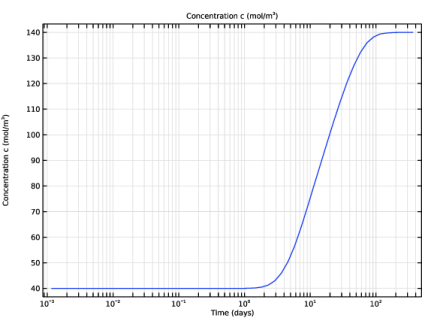
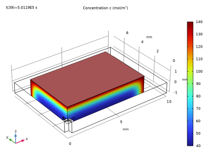
In the Settings window for Surface, click Replace Expression in the upper-right corner of the Expression section. From the menu, choose Component 1 (comp1) > Transport in Solids > Species c > ts.c - Concentration c - mol/m³.
|
|
3
|
|
4
|
|
5
|
|
1
|
|
2
|
|
3
|
Select the Plot checkbox.
|
|
4
|
|
1
|
|
2
|
|
3
|
|
4
|
|
1
|
|
2
|
In the Settings window for 1D Plot Group, type Concentration at Die Location in the Label text field.
|
|
3
|
|
1
|
|
3
|
In the Settings window for Point Graph, click Replace Expression in the upper-right corner of the y-Axis Data section. From the menu, choose Component 1 (comp1) > Transport in Solids > Species c > ts.c - Concentration c - mol/m³.
|
|
4
|
|
1
|
|
2
|
|
3
|
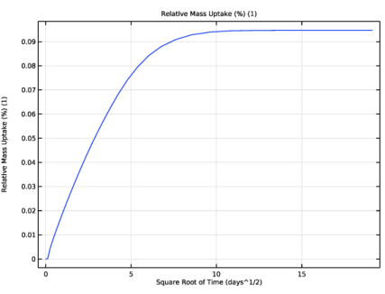
Select the x-axis log scale checkbox.
|
|
4
|
|
5
|
Locate the Plot Settings section.
|
|
6
|
|
7
|
|
1
|
|
2
|
|
3
|
|
4
|
|
1
|
|
2
|
|
4
|
|
5
|
|
6
|
|
1
|
|
2
|
|
3
|
Select the x-axis label checkbox. In the associated text field, type Square Root of Time (days^1/2).
|
|
4
|
|
5
|
|
6
|
|
7
|
|
8
|
|
1
|
|
2
|
Go to the Result Templates window.
|
|
3
|
|
4
|
Click the Add Result Template button in the window toolbar.
|
|
5
|
|
6
|
Click the Add Result Template button in the window toolbar.
|
|
7
|
|
1
|
|
2
|
|
1
|
|
2
|
|
1
|
|
2
|
|
3
|
|
4
|
|
1
|
|
2
|
|
3
|
|
4
|
|
1
|
|
1
|
|
2
|
Go to the Result Templates window.
|
|
3
|
|
4
|
Click the Add Result Template button in the window toolbar.
|
|
5
|
|
1
|
|
2
|
|
1
|
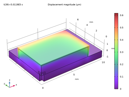
In the Model Builder window, expand the Results > Displacement > Volume 1 node, then click Deformation.
|
|
2
|
|
3
|
|
1
|
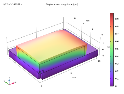
In the Model Builder window, under Results > Displacement right-click Volume 1 and choose Duplicate.
|
|
2
|
|
3
|
|
4
|
|
5
|
Click Replace Expression in the upper-right corner of the Expression section. From the menu, choose Component 1 (comp1) > Shell > Displacement > shell.disp - Displacement magnitude - m.
|
|
6
|
|
7
|
|
1
|
|
2
|
In the Settings window for Deformation, click Replace Expression in the upper-right corner of the Expression section. From the menu, choose Component 1 (comp1) > Shell > Displacement > u2,v2,w2 - Displacement field.
|
|
1
|
|
2
|
|
3
|
|
4
|
|
1
|
|
2
|
|
1
|
|
2
|
|
3
|
|
4
|
|
5
|
|
6
|
|
7
|
|
1
|
|
2
|
|
3
|
|
4
|
|
5
|
|
6
|
|
7
|
Click
|
|
1
|
|
2
|
|
3
|
|
4
|
|
5
|
|
6
|
|
7
|
|
8
|
|
9
|
|
1
|
|
2
|
|
3
|
|
4
|
|
5
|
|
6
|
|
7
|
|
8
|
|
9
|
|
1
|
|
2
|
|
3
|
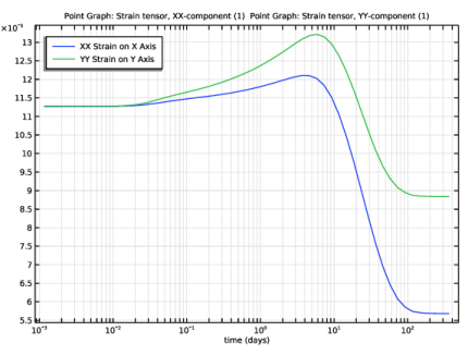
Select the x-axis log scale checkbox.
|
|
4
|
Locate the Plot Settings section.
|
|
5
|
|
6
|
|
7
|
|
1
|
|
2
|
Click
|
|
1
|
|
2
|
|
3
|
Click
|
|
4
|
Browse to the model’s Application Libraries folder and double-click the file pressure_sensor_hygroscopic_swelling_parameters.txt.
|
|
5
|
|
1
|
In the Model Builder window, expand the Component 1 (comp1) > Geometry 1 node, then click Geometry 1.
|
|
2
|
|
3
|
|
1
|
|
2
|
|
3
|
|
4
|
|
5
|
|
6
|
Click to expand the Layers section. In the table, enter the following settings:
|
|
1
|
|
2
|
|
3
|
|
4
|
|
5
|
|
1
|
|
2
|
|
3
|
|
4
|
|
5
|
|
1
|
|
2
|
|
3
|
|
4
|
|
5
|
Select the object blk3 only.
|
|
6
|
Click
|
|
1
|
|
2
|
|
3
|
|
4
|
|
5
|
|
6
|
|
1
|
|
2
|
|
3
|
|
4
|
|
5
|
|
6
|
|
1
|
|
2
|
Select the object blk4 only.
|
|
3
|
|
4
|
|
5
|
Select the object blk5 only.
|
|
6
|
Click
|
|
1
|
|
2
|
|
1
|
|
2
|
|
3
|
|
4
|
|
5
|
Click
|
|
6
|