PDF

Interference Fit Connection in a Mountain Bike Fork
Introduction
Interference fit is a technique used to join two pipes with each other. The smaller pipe, which is slightly larger than the available space in the larger pipe, is cooled down so that it fits. When shrunk, it is fitted into the larger pipe. When the temperature returns to normal, the expansion of the inner pipe will force the outer pipe to expand and the pipes will be pressed against each other. The contact pressure and friction coefficient between the two surfaces determine the strength of the connection.
In this model of a mountain bike fork, the steerer tube is connected to the crown through a shrink fit.
Model Definition
The geometry of the front fork is shown in Figure 1. The damping elements located in the stanchions have been removed from the model since they do not contribute to the structural response during the interference fit mounting.
Figure 1: Front fork.
The entire fork is made out of AISI 4130 steel with the following material data:
Young’s modulus E = 210 GPa
Poisson's ratio ν = 0.29
Density ρ = 7800 kg/m3.
The radial overlap between the two parts is 0.04 mm and the static friction coefficient is assumed to be 0.2.
Results and Discussion
The equivalent stress in the assembly is shown in Figure 2. The stresses on the outer surface are about 300 MPa. Much higher stresses are found below the surface close to the interference fit. Isosurfaces of the equivalent stress are shown in Figure 3. The picture clearly shows that the stress gradient is high around the interference fit.
Figure 2: The equivalent stress caused by the interference fit.
Figure 3: The isosurfaces of the equivalent stress.
The largest tensile and compressive stresses are shown in Figure 4-Figure 5. The largest tensile stress, with a magnitude of about 230 MPa, is located in the crown, while the largest compressive stress, with a magnitude of about -410 MPa, is found in the steerer tube. Since the tube was slightly larger than the available space in the crown, it must shrink, while the crown must expand. The maximum transferable force and moment through the shrink fit is 22 kN and 442 Nm, respectively.
Figure 4: First principal stress.
Figure 5: Third principal stress.
The contact pressure in the interference fit is shown in Figure 6.
Figure 6: Contact pressure.
Notes About the COMSOL Implementation
When analyzing a mounting process, it is common that the two parts are not in contact in the initial configuration. In order to obtain a well-posed model none of the parts can have possible rigid body motions. In the model this is ensured by using a Fixed Constraint on a few boundaries of the crown, and by adding a Stabilization node under the Contact node.
When modeling contact problems like this, where the contacting boundaries have very small relative movements, the performance can be improved by selecting Initial configuration as Mapping method in the Contact pair node. In order to ensure a smooth contact pressure distribution that is not affected by the mesh discretization on the contact boundaries, Force zero initial gap has been selected in the Contact node.
Application Library path: Structural_Mechanics_Module/Contact_and_Friction/mountain_bike_fork
Modeling Instructions
From the File menu, choose New.
New
In the New window, click  Model Wizard.
Model Wizard
1
In the Model Wizard window, click  3D.
2
In the Select Physics tree, select Structural Mechanics > Solid Mechanics (solid).
3
Click Add.
4
Click  Study.
5
In the Select Study tree, select General Studies > Stationary.
6
Geometry 1
Import 1 (imp1)
1
In the Geometry toolbar, click  Import.
2
In the Settings window for Import, locate the Source section.
3
From the Source list, choose COMSOL Multiphysics file.
4
Click  Browse.
5
6
Click  Import.
Form Union (fin)
1
In the Model Builder window, under Component 1 (comp1) > Geometry 1 click Form Union (fin).
2
In the Settings window for Form Union/Assembly, locate the Form Union/Assembly section.
3
From the Action list, choose Form an assembly.
4
From the Frame for identity pairs list, choose Material  (X, Y, Z).
5
In the Geometry toolbar, click  Build All.
Disable the analysis of the geometry as the remaining geometric details can be kept.
6
In the Model Builder window, click Geometry 1.
7
In the Settings window for Geometry, locate the Cleanup section.
8
Clear the Automatic detection of small details checkbox.
Definitions
Identity Boundary Pair 2 (ap2)
1
In the Model Builder window, expand the Component 1 (comp1) > Definitions node, then click Identity Boundary Pair 2 (ap2).
2
In the Settings window for Pair, locate the Pair Type section.
3
Select the Manual control of selections and pair type checkbox.
4
From the Pair type list, choose Contact pair.
5
Locate the Advanced section. From the Mapping method list, choose Initial configuration.
Identity Boundary Pair 3 (ap3)
1
In the Model Builder window, click Identity Boundary Pair 3 (ap3).
2
In the Settings window for Pair, click the  Swap Source and Destination button.
Global Definitions
Parameters 1
1
In the Model Builder window, under Global Definitions click Parameters 1.
2
In the Settings window for Parameters, locate the Parameters section.
3
Materials
Steel
1
In the Model Builder window, under Component 1 (comp1) right-click Materials and choose Blank Material.
2
In the Settings window for Material, type Steel in the Label text field.
3
Locate the Material Contents section. In the table, enter the following settings:
Solid Mechanics (solid)
Contact 1
1
In the Model Builder window, under Component 1 (comp1) > Solid Mechanics (solid) click Contact 1.
2
In the Settings window for Contact, click to expand the Contact Surface Offset and Adjustment section.
3
In the doffset,d text field, type (0.04[mm])*n.
4
Select the Force zero initial gap checkbox.
Friction 1
1
In the Physics toolbar, click  Attributes and choose Friction.
2
In the Settings window for Friction, locate the Friction Parameters section.
3
In the μ text field, type mu.
Contact 1
In the Model Builder window, click Contact 1.
Stabilization 1
In the Physics toolbar, click  Attributes and choose Stabilization.
Fixed Constraint 1
1
In the Physics toolbar, click  Boundaries and choose Fixed Constraint.
2
Symmetry 1
1
In the Physics toolbar, click  Boundaries and choose Symmetry.
2
Mesh 1
Mapped 1
1
In the Mesh toolbar, click  More Generators and choose Mapped.
2
Distribution 1
1
Right-click Mapped 1 and choose Distribution.
2
3
In the Settings window for Distribution, locate the Distribution section.
4
In the Number of elements text field, type 15.
Distribution 2
1
In the Model Builder window, right-click Mapped 1 and choose Distribution.
2
3
In the Settings window for Distribution, locate the Distribution section.
4
From the Distribution type list, choose Predefined.
5
In the Number of elements text field, type 6.
6
In the Element ratio text field, type 2.
7
Select the Reverse direction checkbox.
Distribution 3
1
Right-click Distribution 2 and choose Duplicate.
2
In the Settings window for Distribution, locate the Edge Selection section.
3
4
Click  Remove from Selection.
5
Swept 1
1
In the Mesh toolbar, click  Swept.
2
In the Settings window for Swept, locate the Domain Selection section.
3
From the Geometric entity level list, choose Domain.
4
5
Click to expand the Source Faces section. Select Boundary 166 only.
6
Click to expand the Destination Faces section. Select Boundary 165 only.
Distribution 1
1
Right-click Swept 1 and choose Distribution.
2
In the Settings window for Distribution, locate the Distribution section.
3
In the Number of elements text field, type 10.
Mapped 2
1
In the Mesh toolbar, click  More Generators and choose Mapped.
2
Distribution 1
1
Right-click Mapped 2 and choose Distribution.
2
3
In the Settings window for Distribution, locate the Distribution section.
4
In the Number of elements text field, type 20.
Distribution 2
1
In the Model Builder window, right-click Mapped 2 and choose Distribution.
2
3
In the Settings window for Distribution, locate the Distribution section.
4
From the Distribution type list, choose Predefined.
5
In the Number of elements text field, type 6.
6
In the Element ratio text field, type 2.
Distribution 3
1
Right-click Distribution 2 and choose Duplicate.
2
In the Settings window for Distribution, locate the Edge Selection section.
3
4
Click  Remove from Selection.
5
6
Locate the Distribution section. Select the Reverse direction checkbox.
Swept 2
1
In the Mesh toolbar, click  Swept.
2
In the Settings window for Swept, locate the Domain Selection section.
3
From the Geometric entity level list, choose Domain.
4
Distribution 1
1
Right-click Swept 2 and choose Distribution.
2
In the Settings window for Distribution, locate the Distribution section.
3
In the Number of elements text field, type 15.
Free Tetrahedral 1
1
In the Mesh toolbar, click  Free Tetrahedral.
2
In the Settings window for Free Tetrahedral, locate the Domain Selection section.
3
From the Geometric entity level list, choose Domain.
4
Size 1
1
Right-click Free Tetrahedral 1 and choose Size.
2
In the Settings window for Size, locate the Element Size section.
3
From the Predefined list, choose Fine.
Free Tetrahedral 2
1
In the Mesh toolbar, click  Free Tetrahedral.
2
In the Settings window for Free Tetrahedral, locate the Domain Selection section.
3
From the Geometric entity level list, choose Domain.
4
Distribution 1
1
Right-click Free Tetrahedral 2 and choose Distribution.
2
3
In the Settings window for Distribution, locate the Distribution section.
4
In the Number of elements text field, type 10.
Size 1
In the Model Builder window, right-click Free Tetrahedral 2 and choose Size.
Size 2
1
Right-click Free Tetrahedral 2 and choose Size.
2
In the Settings window for Size, locate the Geometric Entity Selection section.
3
From the Geometric entity level list, choose Boundary.
4
5
Locate the Element Size section. From the Predefined list, choose Finer.
Size 1
1
In the Model Builder window, click Size 1.
2
In the Settings window for Size, locate the Element Size section.
3
Click the Custom button.
4
Locate the Element Size Parameters section.
5
Select the Minimum element size checkbox. In the associated text field, type 0.011.
6
Click  Build All.
Study 1
Step 1: Stationary
1
In the Model Builder window, under Study 1 click Step 1: Stationary.
2
In the Settings window for Stationary, click to expand the Study Extensions section.
3
Select the Auxiliary sweep checkbox.
4
5
Solution 1 (sol1)
1
In the Study toolbar, click  Show Default Solver.
Since the contact surface is assumed to be established, you can use less conservative solver settings to speed up the computations.
2
In the Model Builder window, expand the Solution 1 (sol1) node.
3
In the Model Builder window, expand the Study 1 > Solver Configurations > Solution 1 (sol1) > Stationary Solver 1 node, then click Fully Coupled 1.
4
In the Settings window for Fully Coupled, click to expand the Method and Termination section.
5
From the Nonlinear method list, choose Automatic (Newton).
6
In the Study toolbar, click  Compute.
Set default units for result presentation.
Results
Preferred Units 1
1
In the Results toolbar, click  Configurations and choose Preferred Units.
2
In the Settings window for Preferred Units, locate the Units section.
3
Click  Add Physical Quantity.
4
In the Physical Quantity dialog, select Solid Mechanics > Stress tensor (N/m^2) in the tree.
5
6
In the Settings window for Preferred Units, locate the Units section.
7
8
Select the Apply conversions to expressions with the same dimensions checkbox.
9
Click  Apply.
Mirror 3D 1
1
In the Model Builder window, expand the Results > Datasets node.
2
Right-click Results > Datasets and choose More 3D Datasets > Mirror 3D.
Stress (solid)
1
In the Settings window for 3D Plot Group, locate the Data section.
2
From the Dataset list, choose Mirror 3D 1.
Volume 1
1
In the Model Builder window, expand the Stress (solid) node, then click Volume 1.
2
In the Stress (solid) toolbar, click  Plot.
Stress (solid)
1
In the Model Builder window, click Stress (solid).
2
In the Settings window for 3D Plot Group, locate the Plot Settings section.
3
From the View list, choose View 3D 2.
4
In the Stress (solid) toolbar, click  Plot.
Use the mouse buttons to zoom in on the region around the interference fit. When done, lock the camera:
5
Click  Go to Source.
View 3D 2
1
In the Model Builder window, under Results > Views click View 3D 2.
2
In the Settings window for View 3D, locate the View section.
3
Select the Lock camera checkbox.
Equivalent Stress, Isosurface
1
In the Results toolbar, click  3D Plot Group.
2
In the Settings window for 3D Plot Group, type Equivalent Stress, Isosurface in the Label text field.
3
Locate the Data section. From the Dataset list, choose Mirror 3D 1.
Isosurface 1
1
Right-click Equivalent Stress, Isosurface and choose Isosurface.
2
In the Settings window for Isosurface, click Replace Expression in the upper-right corner of the Expression section. From the menu, choose Component 1 (comp1) > Solid Mechanics > Stress > solid.misesGp - von Mises stress - N/m².
3
Locate the Levels section. From the Entry method list, choose Levels.
4
In the Levels text field, type range(100,50,400).
Result Templates
1
In the Home toolbar, click  Result Templates to open the Result Templates window.
2
Go to the Result Templates window.
3
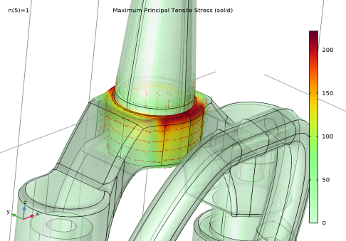
In the tree, select Study 1/Solution 1 (sol1) > Solid Mechanics > Maximum Principal Tensile Stress (solid).
4
Click the Add Result Template button in the window toolbar.
Result Templates
1
Go to the Result Templates window.
2
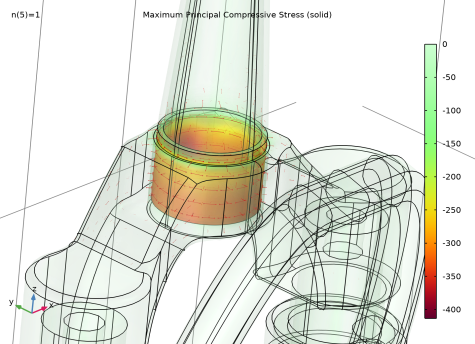
In the tree, select Study 1/Solution 1 (sol1) > Solid Mechanics > Maximum Principal Compressive Stress (solid).
3
Click the Add Result Template button in the window toolbar.
Results
Maximum Principal Compressive Stress (solid)
In the Home toolbar, click  Result Templates to close the Result Templates window.
Maximum Principal Tensile Stress (solid)
1
In the Model Builder window, click Maximum Principal Tensile Stress (solid).
2
In the Settings window for 3D Plot Group, locate the Data section.
3
From the Dataset list, choose Mirror 3D 1.
4
Locate the Plot Settings section. From the View list, choose View 3D 2.
5
In the Maximum Principal Tensile Stress (solid) toolbar, click  Plot.
Transparency 1
1
In the Model Builder window, expand the Maximum Principal Tensile Stress (solid) node.
2
Right-click Surface 1 and choose Transparency.
3
In the Settings window for Transparency, locate the Transparency section.
4
Find the Transparency subsection. From the Input list, choose Expression.
5
In the Expression text field, type max(solid.sp1Gp,0).
6
In the Maximum transparency text field, type 0.5.
7
Select the Reverse checkbox.
Principal Stress Surface 1
1
In the Model Builder window, under Results > Maximum Principal Tensile Stress (solid) click Principal Stress Surface 1.
2
In the Settings window for Principal Stress Surface, locate the Positioning section.
3
In the Number of points text field, type 10000.
4
Locate the Coloring and Style section.
5
Select the Scale factor checkbox. In the associated text field, type 2E-11.
Maximum Principal Compressive Stress (solid)
1
In the Model Builder window, under Results click Maximum Principal Compressive Stress (solid).
2
In the Settings window for 3D Plot Group, locate the Data section.
3
From the Dataset list, choose Mirror 3D 1.
4
Locate the Plot Settings section. From the View list, choose View 3D 2.
5
In the Maximum Principal Compressive Stress (solid) toolbar, click  Plot.
Transparency 1
1
In the Model Builder window, expand the Maximum Principal Compressive Stress (solid) node.
2
Right-click Surface 1 and choose Transparency.
3
In the Settings window for Transparency, locate the Transparency section.
4
Find the Transparency subsection. From the Input list, choose Expression.
5
In the Expression text field, type min(solid.sp3Gp,0).
6
In the Maximum transparency text field, type 0.9.
Principal Stress Surface 1
1
In the Model Builder window, under Results > Maximum Principal Compressive Stress (solid) click Principal Stress Surface 1.
2
In the Settings window for Principal Stress Surface, locate the Coloring and Style section.
3
Select the Scale factor checkbox.
4
Locate the Positioning section. In the Number of points text field, type 10000.
5
Locate the Coloring and Style section. In the Scale factor text field, type 8E-12.
Contact Pressure
1
In the Results toolbar, click  3D Plot Group.
2
In the Settings window for 3D Plot Group, type Contact Pressure in the Label text field.
3
Locate the Data section. From the Dataset list, choose Mirror 3D 1.
Surface 1
1
Right-click Contact Pressure and choose Surface.
2
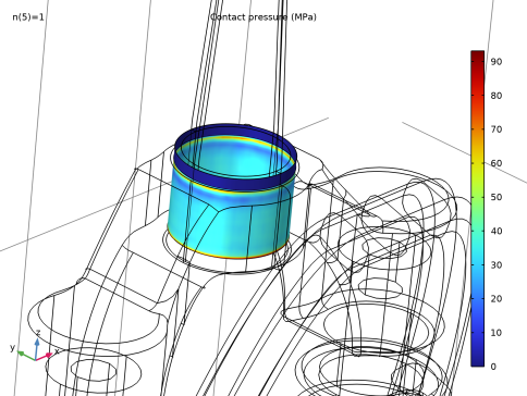
In the Settings window for Surface, click Replace Expression in the upper-right corner of the Expression section. From the menu, choose Component 1 (comp1) > Solid Mechanics > Contact > solid.Tn - Contact pressure - N/m².
Unlock the camera view.
View 3D 2
1
In the Model Builder window, under Results > Views click View 3D 2.
2
In the Settings window for View 3D, locate the View section.
3
Clear the Lock camera checkbox.
Transferable Loads
1
In the Results toolbar, click  More Derived Values and choose Integration > Surface Integration.
2
In the Settings window for Surface Integration, type Transferable Loads in the Label text field.
3
4
Locate the Data section. From the Parameter selection (n) list, choose Last.
5
Locate the Expressions section. In the table, enter the following settings:
6
Click  Evaluate.