PDF

Micromechanical Model of a Piezoelectric Fiber Composite
Introduction
The monolithic piezoelectric materials found their use in many applications like sensors, actuators and transducers. The advancement of technology demands more advanced materials, which increases the usability and applications of composite piezoelectric materials. Compared to monolithic piezoelectric materials, composite piezoelectric material offers superior mechanical and thermal properties along with customized piezoelectric properties. These composite piezoelectric materials need complete set of constitutive properties in order to be analyzed numerically. A micromechanical analysis is one of the tools to obtain the homogenized electromechanical properties of piezoelectric composite materials.
The model is a benchmark example taken from the Ref. 1. In this example, a simplified micromechanical model of a unit cell with periodic boundary conditions is analyzed. The unit cell represents one type of piezocomposite from Ref. 1, which is a square-diagonal arrangement of fibers in a matrix. The homogenized electromechanical properties of the composite material are computed based on the individual properties of the fiber and matrix, fiber volume fraction, and the poling directions. The fibers in composite material is made of PZT-7A material, while the matrix is made of Barium Titanate. The fiber volume fraction is varied to check its effect on the homogenized properties. The poling directions of the matrix and fiber are parallel and aligned to the fiber axis.
Model Definition
The unit cell of cylindrical fibers embedded in a matrix is shown in Figure 1. The fiber radius is computed based on a parameterized fiber volume fraction.
Figure 1: Geometry of the unit cell with a PZT-7A fibers in a Barium Titanate matrix.
Fiber and Matrix Properties
The fibers are made of PZT-7A material, and the matrix is made of Barium Titanate material, for which the built-in materials from the COMSOL Multiphysics material library are used.
The permittivity tensor at constant strain given in Ref. 1 for both materials is incorrect. It seems that the authors have instead used permittivity tensor at constant stress for the stress-charge formulation. The built-in materials in the COMSOL Multiphysics use correct permittivity or relative permittivity tensor, which in turn changes the result values of the homogenized permittivity tensor.
Results and Discussion
Figure 2 through Figure 6 show the homogenized elasticity tensor components for different fiber volume fractions. Some of the components increase linearly, while others decrease linearly with increase in the fiber volume fraction. The results very closely match those presented in Ref. 1 (see figure 4).
Figure 7 and Figure 8 show the homogenized piezoelectric coupling tensor components for different fiber volume fractions. Again, the results very closely match those presented in Ref. 1 (see figure 5). Figure 9 and Figure 10 show the homogenized permittivity tensor components for different fiber volume fractions. The homogenized permittivity tensor value varies with the fiber volume fraction in the same fashion as reported in Ref. 1, but the values do not match because the authors have used the permittivity tensor at constant stress for the fiber and matrix material.
Table 1, Table 2, and Table 3 show the nonzero components of the homogenized elasticity, homogenized piezoelectric coupling, and homogenized permittivity tensor, respectively. The values are for 70% fiber volume fraction. It is clear that the values presented in the reference paper closely match the values obtained with COMSOL Multiphysics. However, a match is not possible for the homogenized permittivity tensor because the authors used erroneous material inputs. In the current example, if one uses the permittivity tensor given by the authors then one gets exactly same homogenized permittivity tensor as presented in Ref. 1.
c11
c12
c13
c22
c23
c33
c44
c55
c66
e15
e24
e31
e32
e33
k11
k22
k33
Figure 2: Homogenized elasticity tensor component 11 versus fiber volume fraction.
Figure 3: Homogenized elasticity tensor component 33 versus fiber volume fraction.
Figure 4: Homogenized elasticity tensor component 44 versus fiber volume fraction.
Figure 5: Homogenized elasticity tensor component 12 versus fiber volume fraction.
Figure 6: Homogenized elasticity tensor component 23 versus fiber volume fraction.
Figure 7: Homogenized piezoelectric coupling tensor component 31 versus fiber volume fraction.
Figure 8: Homogenized piezoelectric coupling tensor component 33 versus fiber volume fraction.
Figure 9: Homogenized permittivity tensor component 11 versus fiber volume fraction.
Figure 10: Homogenized permittivity tensor component 33 versus fiber volume fraction.
Notes About the COMSOL Implementation
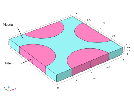
To get the homogenized elastic and piezoelectric coupling tensor, the Cell Periodicity node in the Solid Mechanics interface is used to apply periodic boundary conditions to the three pairs of faces of the unit cell.
In order to get homogenized permittivity tensor, the periodic conditions are applied using Pointwise Constraint nodes in the Electrostatics interface. The Piezoelectricity multiphysics coupling is needed to couple the mechanical and electrical effects.
The Cell Periodicity node has three action buttons in the toolbar of the section called Periodicity Type: Create Load Groups and Study, Create Material by Value, and Create Material by Reference. The action button Create Load Groups and Study generates load groups and a stationary study with load cases. The action button Create Material by Value generates a Global Material with homogenized material properties, with material properties as numbers. The action button Create Material by Reference generates a Global Material with homogenized material properties, with material properties as variables. The action buttons are active depending on the choices in the Periodicity Type and Calculate Average Properties lists.
The Create Load Groups and Study button does not generate a parametric study by default. In many situations, a parametric study is needed, and the homogenized elasticity matrix D needs to be based on the tag of the parametric solution. To do this use the given options in the Advanced section of the feature.
Reference
1. R.K. Gupta and T.A. Venkatesh, “Electromechanical response of 1-3 piezoelectric composites: Effect of poling characteristics,” J. Appl. Phys., vol. 98, no. 5, p. 054102,2005.
Application Library path: Structural_Mechanics_Module/Material_Models/micromechanical_model_of_a_piezoelectric_composite
Modeling Instructions
From the File menu, choose New.
New
In the New window, click  Model Wizard.
Model Wizard
1
In the Model Wizard window, click  3D.
2
In the Select Physics tree, select Structural Mechanics > Electromagnetics–Structure Interaction > Piezoelectricity > Piezoelectricity, Solid.
3
Click Add.
4
Global Definitions
Parameters 1
1
In the Model Builder window, under Global Definitions click Parameters 1.
2
In the Settings window for Parameters, locate the Parameters section.
3
Geometry 1
Block 1 (blk1)
1
In the Geometry toolbar, click  Block.
2
In the Settings window for Block, locate the Size and Shape section.
3
In the Width text field, type W.
4
In the Depth text field, type D.
5
In the Height text field, type H.
6
Click  Build Selected.
Work Plane 1 (wp1)
In the Geometry toolbar, click  Work Plane.
Work Plane 1 (wp1) > Plane Geometry
In the Model Builder window, click Plane Geometry.
Work Plane 1 (wp1) > Circle 1 (c1)
1
In the Work Plane toolbar, click  Circle.
2
In the Settings window for Circle, locate the Size and Shape section.
3
In the Radius text field, type r_f.
4
In the Sector angle text field, type 180.
5
Locate the Position section. In the yw text field, type D/2.
6
Locate the Rotation Angle section. In the Rotation text field, type -90.
7
Click  Build Selected.
Work Plane 1 (wp1) > Circle 2 (c2)
1
In the Work Plane toolbar, click  Circle.
2
In the Settings window for Circle, locate the Size and Shape section.
3
In the Radius text field, type r_f.
4
In the Sector angle text field, type 180.
5
Locate the Position section. In the xw text field, type W.
6
In the yw text field, type D/2.
7
Locate the Rotation Angle section. In the Rotation text field, type 90.
8
Click  Build Selected.
Work Plane 1 (wp1) > Circle 3 (c3)
1
In the Work Plane toolbar, click  Circle.
2
In the Settings window for Circle, locate the Size and Shape section.
3
In the Radius text field, type r_f.
4
In the Sector angle text field, type 180.
5
Locate the Position section. In the xw text field, type W/2.
6
In the yw text field, type D.
7
Locate the Rotation Angle section. In the Rotation text field, type 180.
8
Click  Build Selected.
Work Plane 1 (wp1) > Circle 4 (c4)
1
In the Work Plane toolbar, click  Circle.
2
In the Settings window for Circle, locate the Size and Shape section.
3
In the Radius text field, type r_f.
4
In the Sector angle text field, type 180.
5
Locate the Position section. In the xw text field, type W/2.
6
Click  Build Selected.
Fiber
1
In the Model Builder window, right-click Geometry 1 and choose Extrude.
2
In the Settings window for Extrude, locate the Distances section.
3
4
In the Label text field, type Fiber.
5
Locate the Selections of Resulting Entities section. Select the Resulting objects selection checkbox.
6
From the Color list, choose None or — if you are running the cross-platform desktop —Custom. On the cross-platform desktop, click the Color button.
7
Click Define custom colors.
8
9
Click Add to custom colors.
10
Click Show color palette only or OK on the cross-platform desktop.
11
Click  Build Selected.
Matrix
1
In the Geometry toolbar, click  Booleans and Partitions and choose Difference.
2
In the Settings window for Difference, type Matrix in the Label text field.
3
4
Locate the Difference section. Click to select the  Activate Selection toggle button for Objects to subtract.
5
From the Objects to subtract list, choose Fiber.
6
Select the Keep objects to subtract checkbox.
7
Locate the Selections of Resulting Entities section. Select the Resulting objects selection checkbox.
8
From the Color list, choose None or — if you are running the cross-platform desktop —Custom. On the cross-platform desktop, click the Color button.
9
Click Define custom colors.
10
11
Click Add to custom colors.
12
Click Show color palette only or OK on the cross-platform desktop.
Form Union (fin)
In the Geometry toolbar, click  Build All.
Pair 1, Source
1
In the Geometry toolbar, click  Selections and choose Box Selection.
2
In the Settings window for Box Selection, locate the Geometric Entity Level section.
3
From the Level list, choose Boundary.
4
In the Label text field, type Pair 1, Source.
5
Locate the Box Limits section. In the x maximum text field, type 0.
6
Locate the Output Entities section. From the Include entity if list, choose Entity inside box.
Pair 1, Destination
1
In the Geometry toolbar, click  Selections and choose Box Selection.
2
In the Settings window for Box Selection, locate the Geometric Entity Level section.
3
From the Level list, choose Boundary.
4
In the Label text field, type Pair 1, Destination.
5
Locate the Box Limits section. In the x minimum text field, type W.
6
Locate the Output Entities section. From the Include entity if list, choose Entity inside box.
Pair 2, Source
1
In the Geometry toolbar, click  Selections and choose Box Selection.
2
In the Settings window for Box Selection, locate the Geometric Entity Level section.
3
From the Level list, choose Boundary.
4
In the Label text field, type Pair 2, Source.
5
Locate the Box Limits section. In the y maximum text field, type 0.
6
Locate the Output Entities section. From the Include entity if list, choose Entity inside box.
Pair 2, Destination
1
In the Geometry toolbar, click  Selections and choose Box Selection.
2
In the Settings window for Box Selection, locate the Geometric Entity Level section.
3
From the Level list, choose Boundary.
4
In the Label text field, type Pair 2, Destination.
5
Locate the Box Limits section. In the y minimum text field, type D.
6
Locate the Output Entities section. From the Include entity if list, choose Entity inside box.
Pair 3, Source
1
In the Geometry toolbar, click  Selections and choose Box Selection.
2
In the Settings window for Box Selection, locate the Geometric Entity Level section.
3
From the Level list, choose Boundary.
4
In the Label text field, type Pair 3, Source.
5
Locate the Box Limits section. In the z maximum text field, type 0.
6
Locate the Output Entities section. From the Include entity if list, choose Entity inside box.
Pair 3, Destination
1
In the Geometry toolbar, click  Selections and choose Box Selection.
2
In the Settings window for Box Selection, locate the Geometric Entity Level section.
3
From the Level list, choose Boundary.
4
In the Label text field, type Pair 3, Destination.
5
Locate the Box Limits section. In the z minimum text field, type H.
6
Locate the Output Entities section. From the Include entity if list, choose Entity inside box.
Pair 1
1
In the Geometry toolbar, click  Selections and choose Union Selection.
2
In the Settings window for Union Selection, locate the Geometric Entity Level section.
3
From the Level list, choose Boundary.
4
Locate the Input Entities section. Click  Add.
5
In the Add dialog, in the Selections to add list, choose Pair 1, Source and Pair 1, Destination.
6
7
In the Settings window for Union Selection, type Pair 1 in the Label text field.
Pair 2
1
In the Geometry toolbar, click  Selections and choose Union Selection.
2
In the Settings window for Union Selection, locate the Geometric Entity Level section.
3
From the Level list, choose Boundary.
4
Locate the Input Entities section. Click  Add.
5
In the Add dialog, in the Selections to add list, choose Pair 2, Source and Pair 2, Destination.
6
7
In the Settings window for Union Selection, type Pair 2 in the Label text field.
Pair 3
1
In the Geometry toolbar, click  Selections and choose Union Selection.
2
In the Settings window for Union Selection, locate the Geometric Entity Level section.
3
From the Level list, choose Boundary.
4
Locate the Input Entities section. Click  Add.
5
In the Add dialog, in the Selections to add list, choose Pair 3, Source and Pair 3, Destination.
6
7
In the Settings window for Union Selection, type Pair 3 in the Label text field.
Add Material
1
In the Home toolbar, click  Add Material to open the Add Material window.
2
Go to the Add Material window.
3
In the tree, select Piezoelectric > Barium Titanate (poled).
4
Right-click and choose Add to Component 1 (comp1).
Materials
Matrix: Barium Titanate (poled)
1
In the Model Builder window, under Component 1 (comp1) > Materials click Barium Titanate (poled) (mat1).
2
In the Settings window for Material, type Matrix: Barium Titanate (poled) in the Label text field.
3
Locate the Geometric Entity Selection section. From the Selection list, choose Matrix.
Add Material
1
Go to the Add Material window.
2
In the tree, select Piezoelectric > Lead Zirconate Titanate (PZT-7A).
3
Right-click and choose Add to Component 1 (comp1).
4
In the Materials toolbar, click  Add Material to close the Add Material window.
Materials
Fiber: Lead Zirconate Titanate (PZT-7A)
1
In the Settings window for Material, type Fiber: Lead Zirconate Titanate (PZT-7A) in the Label text field.
2
Locate the Geometric Entity Selection section. From the Selection list, choose Fiber.
Solid Mechanics (solid)
Cell Periodicity 1
1
In the Physics toolbar, click  Domains and choose Cell Periodicity.
2
In the Settings window for Cell Periodicity, locate the Periodicity Settings section.
3
From the Boundary conditions list, choose Average strain.
4
Locate the Effective Properties section. Select the Compute elasticity matrix, Voigt notation checkbox.
Boundary Pair 1
1
In the Physics toolbar, click  Attributes and choose Boundary Pair.
2
In the Settings window for Boundary Pair, locate the Boundary Selection section.
3
From the Selection list, choose Pair 1.
4
Right-click Boundary Pair 1 and choose Manual Destination Selection.
5
Locate the Destination Selection section. From the Selection list, choose Pair 1, Destination.
Cell Periodicity 1
In the Model Builder window, click Cell Periodicity 1.
Boundary Pair 2
1
In the Physics toolbar, click  Attributes and choose Boundary Pair.
2
In the Settings window for Boundary Pair, locate the Boundary Selection section.
3
From the Selection list, choose Pair 2.
4
Right-click Boundary Pair 2 and choose Manual Destination Selection.
5
Locate the Destination Selection section. From the Selection list, choose Pair 2, Destination.
Cell Periodicity 1
In the Model Builder window, click Cell Periodicity 1.
Boundary Pair 3
1
In the Physics toolbar, click  Attributes and choose Boundary Pair.
2
In the Settings window for Boundary Pair, locate the Boundary Selection section.
3
From the Selection list, choose Pair 3.
4
Right-click Boundary Pair 3 and choose Manual Destination Selection.
5
Locate the Destination Selection section. From the Selection list, choose Pair 3, Destination.
With the Average strain option selected in the Cell Periodicity feature, appropriate load groups, a study, and a material with computed elastic properties can be generated automatically. To create load groups and a study node, click the Create Load Groups and Study button in the section toolbar.
Cell Periodicity 1
To create a parametric study, use the options in the Advanced section of the feature. To see this section, activate the Advanced Physics option.
1
Click the  Show More Options button in the Model Builder toolbar.
2
In the Show More Options dialog, in the tree, select the checkbox for the node Physics > Advanced Physics Options.
3
4
In the Model Builder window, click Cell Periodicity 1.
5
In the Settings window for Cell Periodicity, click to expand the Advanced section.
6
From the Add parametric sweep list, choose Yes.
7
In the Parameters table, enter the following settings:
8
Click Automated Model Setup in the upper-right corner of the Periodicity Settings section. From the menu, choose Create Load Groups and Study.
To compute the homogenized permittivity tensor, three additional electric potential load cases are needed. Add three Load Group nodes under the Load Groups for Cell Periodicity group.
Global Definitions
Load Group 1
1
In the Model Builder window, expand the Global Definitions > Load and Constraint Groups node.
2
Right-click Load Groups for Cell Periodicity and choose Load Group.
Load Group 2
Right-click Load Groups for Cell Periodicity and choose Load Group.
Load Group 3
Right-click Load Groups for Cell Periodicity and choose Load Group.
The periodic conditions in the Electrostatics interface need to be implemented using Pointwise Constraint features. To define the constraints, add three General Extrusion operators.
Definitions
General Extrusion 1 (genext1)
1
In the Definitions toolbar, click  Nonlocal Couplings and choose General Extrusion.
2
In the Settings window for General Extrusion, locate the Source Selection section.
3
From the Geometric entity level list, choose Boundary.
4
From the Selection list, choose Pair 1, Source.
5
Click to expand the Advanced section. From the Mesh search method list, choose Closest point.
General Extrusion 2 (genext2)
1
Right-click General Extrusion 1 (genext1) and choose Duplicate.
2
In the Settings window for General Extrusion, locate the Source Selection section.
3
From the Selection list, choose Pair 2, Source.
General Extrusion 3 (genext3)
1
Right-click General Extrusion 2 (genext2) and choose Duplicate.
2
In the Settings window for General Extrusion, locate the Source Selection section.
3
From the Selection list, choose Pair 3, Source.
4
Click the  Show More Options button in the Model Builder toolbar.
5
In the Show More Options dialog, in the tree, select the checkbox for the node Physics > Equation Contributions.
6
Electrostatics (es)
Periodic Condition, Boundary Pair 1
1
In the Physics toolbar, click  Boundaries and choose Pointwise Constraint.
2
In the Settings window for Pointwise Constraint, type Periodic Condition, Boundary Pair 1 in the Label text field.
3
Locate the Boundary Selection section. From the Selection list, choose Pair 1, Destination.
4
Locate the Pointwise Constraint section. In the Constraint expression text field, type V+group.lg1*1[V/m]*W-genext1(V).
Periodic Condition, Boundary Pair 2
1
Right-click Periodic Condition, Boundary Pair 1 and choose Duplicate.
2
In the Settings window for Pointwise Constraint, type Periodic Condition, Boundary Pair 2 in the Label text field.
3
Locate the Boundary Selection section. From the Selection list, choose Pair 2, Destination.
4
Locate the Pointwise Constraint section. In the Constraint expression text field, type V+group.lg2*1[V/m]*D-genext2(V).
Periodic Condition, Boundary Pair 3
1
Right-click Periodic Condition, Boundary Pair 2 and choose Duplicate.
2
In the Settings window for Pointwise Constraint, type Periodic Condition, Boundary Pair 3 in the Label text field.
3
Locate the Boundary Selection section. From the Selection list, choose Pair 3, Destination.
4
Locate the Pointwise Constraint section. In the Constraint expression text field, type V+group.lg3*1[V/m]*H-genext3(V).
Ground 1
1
In the Physics toolbar, click  Points and choose Ground.
2
Definitions
Integration 1 (intop1)
1
In the Definitions toolbar, click  Nonlocal Couplings and choose Integration.
2
In the Settings window for Integration, locate the Source Selection section.
3
From the Selection list, choose All domains.
Variables 1
1
In the Model Builder window, right-click Definitions and choose Variables.
2
In the Settings window for Variables, locate the Variables section.
3
Click  Load from File.
4
Browse to the model’s Application Libraries folder and double-click the file micromechanical_model_of_a_piezoelectric_composite_variables.txt.
Mesh 1
1
In the Model Builder window, under Component 1 (comp1) click Mesh 1.
2
In the Settings window for Mesh, locate the Physics-Controlled Mesh section.
3
From the Element size list, choose Finer.
4
Click  Build All.
Add three load cases corresponding to the three additional electric potential load cases.
Cell Periodicity Study
Step 1: Stationary
1
In the Model Builder window, expand the Cell Periodicity Study node, then click Step 1: Stationary.
2
In the Settings window for Stationary, locate the Study Extensions section.
3
Click  Add three times.
4
5
In the Study toolbar, click  Compute.
When plotting the computed elasticity matrix elements in 1D plot groups, the load case in the parameter selection is irrelevant.
Results
Homogenized Elasticity Tensor Component 11
1
In the Results toolbar, click  1D Plot Group.
2
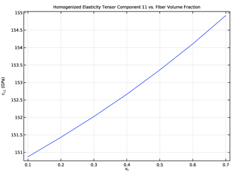
In the Settings window for 1D Plot Group, type Homogenized Elasticity Tensor Component 11 in the Label text field.
3
Locate the Data section. From the Dataset list, choose Cell Periodicity Study/Solution 2 (solidcp1solp).
4
From the Parameter selection (Load case) list, choose First.
5
Click to expand the Title section. From the Title type list, choose Manual.
6
In the Title text area, type Homogenized Elasticity Tensor Component 11 vs. Fiber Volume Fraction.
7
Locate the Plot Settings section.
8
Select the x-axis label checkbox. In the associated text field, type v<sub>f</sub>.
9
Select the y-axis label checkbox. In the associated text field, type c<sub>11</sub> (GPa).
10
Locate the Legend section. Clear the Show legends checkbox.
Global 1
1
Right-click Homogenized Elasticity Tensor Component 11 and choose Global.
2
In the Settings window for Global, locate the y-Axis Data section.
3
4
Locate the x-Axis Data section. From the Axis source data list, choose v_f.
5
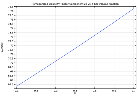
Click to expand the Coloring and Style section. Duplicate or add this plot group five times in order to plot the remaining elastic properties. The labels, titles, and the expressions to be defined in the Global 1 node are shown in the table below.
Homogenized Piezoelectric Coupling Tensor Component 31
1
In the Results toolbar, click  1D Plot Group.
2
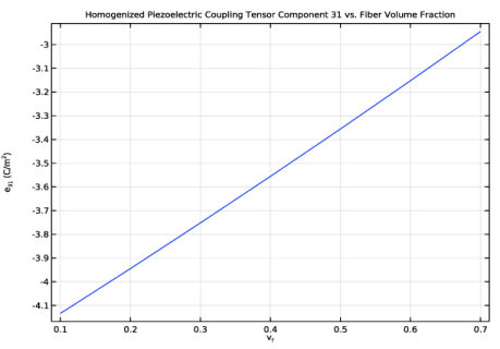
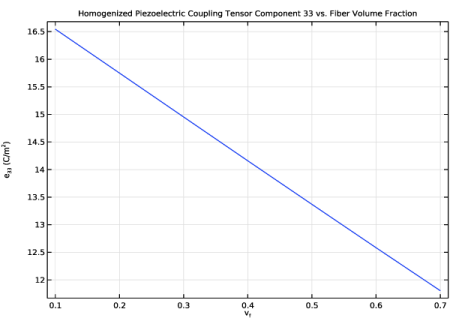
In the Settings window for 1D Plot Group, type Homogenized Piezoelectric Coupling Tensor Component 31 in the Label text field.
3
Locate the Data section. From the Dataset list, choose Cell Periodicity Study/Solution 2 (solidcp1solp).
4
From the Parameter selection (Load case) list, choose First.
5
Locate the Title section. From the Title type list, choose Manual.
6
In the Title text area, type Homogenized Piezoelectric Coupling Tensor Component 31 vs. Fiber Volume Fraction.
7
Locate the Plot Settings section.
8
Select the x-axis label checkbox. In the associated text field, type v<sub>f</sub>.
9
Select the y-axis label checkbox. In the associated text field, type e<sub>31</sub> (C/m<sup>2</sup>).
10
Locate the Legend section. Clear the Show legends checkbox.
Global 1
1
Right-click Homogenized Piezoelectric Coupling Tensor Component 31 and choose Global.
2
In the Settings window for Global, locate the y-Axis Data section.
3
4
Locate the x-Axis Data section. From the Axis source data list, choose v_f.
5
Homogenized Permittivity Tensor Component 11
1
In the Results toolbar, click  1D Plot Group.
2
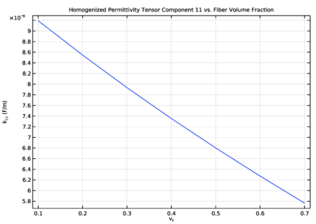
In the Settings window for 1D Plot Group, type Homogenized Permittivity Tensor Component 11 in the Label text field.
3
Locate the Data section. From the Dataset list, choose Cell Periodicity Study/Solution 2 (solidcp1solp).
4
From the Parameter selection (Load case) list, choose First.
5
Locate the Title section. From the Title type list, choose Manual.
6
In the Title text area, type Homogenized Permittivity Tensor Component 11 vs. Fiber Volume Fraction.
7
Locate the Plot Settings section.
8
Select the x-axis label checkbox. In the associated text field, type v<sub>f</sub>.
9
Select the y-axis label checkbox. In the associated text field, type k<sub>11</sub> (F/m).
10
Locate the Legend section. Clear the Show legends checkbox.
Global 1
1
Right-click Homogenized Permittivity Tensor Component 11 and choose Global.
2
In the Settings window for Global, locate the y-Axis Data section.
3
4
Locate the x-Axis Data section. From the Axis source data list, choose v_f.
5
Homogenized Elasticity Tensor (70% Fiber Volume Fraction)
1
In the Model Builder window, under Results click Effective Material Properties (Cell Periodicity Study).
2
In the Settings window for Evaluation Group, type Homogenized Elasticity Tensor (70% Fiber Volume Fraction) in the Label text field.
Homogenized Piezoelectric Coupling Tensor (70% Fiber Volume Fraction)
1
In the Results toolbar, click  Evaluation Group.
2
In the Settings window for Evaluation Group, type Homogenized Piezoelectric Coupling Tensor (70% Fiber Volume Fraction) in the Label text field.
3
Locate the Data section. From the Dataset list, choose Cell Periodicity Study/Solution 2 (solidcp1solp).
4
From the Parameter selection (v_f) list, choose Last.
5
From the Parameter selection (Load case) list, choose Last.
6
Click to expand the Format section. From the Include parameters list, choose Off.
7
From the Concatenation list, choose Vertical.
Global Evaluation 1
1
Right-click Homogenized Piezoelectric Coupling Tensor (70% Fiber Volume Fraction) and choose Global Evaluation.
2
In the Settings window for Global Evaluation, locate the Expressions section.
3
Global Evaluation 2
1
Right-click Global Evaluation 1 and choose Duplicate.
2
In the Settings window for Global Evaluation, locate the Expressions section.
3
Global Evaluation 3
1
Right-click Global Evaluation 2 and choose Duplicate.
2
In the Settings window for Global Evaluation, locate the Expressions section.
3
4
In the Homogenized Piezoelectric Coupling Tensor (70% Fiber Volume Fraction) toolbar, click  Evaluate.
Homogenized Permittivity Tensor (70% Fiber Volume Fraction)
1
In the Results toolbar, click  Evaluation Group.
2
In the Settings window for Evaluation Group, type Homogenized Permittivity Tensor (70% Fiber Volume Fraction) in the Label text field.
3
Locate the Data section. From the Dataset list, choose Cell Periodicity Study/Solution 2 (solidcp1solp).
4
From the Parameter selection (v_f) list, choose Last.
5
From the Parameter selection (Load case) list, choose Last.
6
Locate the Format section. From the Include parameters list, choose Off.
7
From the Concatenation list, choose Vertical.
Global Evaluation 1
1
Right-click Homogenized Permittivity Tensor (70% Fiber Volume Fraction) and choose Global Evaluation.
2
In the Settings window for Global Evaluation, locate the Expressions section.
3
Global Evaluation 2
1
Right-click Global Evaluation 1 and choose Duplicate.
2
In the Settings window for Global Evaluation, locate the Expressions section.
3
Global Evaluation 3
1
Right-click Global Evaluation 2 and choose Duplicate.
2
In the Settings window for Global Evaluation, locate the Expressions section.
3
4
In the Homogenized Permittivity Tensor (70% Fiber Volume Fraction) toolbar, click  Evaluate.