PDF

Micromechanical Model of a Fiber Composite
Introduction
The use of fiber-reinforced composites is increasing in various industries like automotive, aerospace, infrastructure, and many more. The accuracy of structural and thermal analyses relies on an accurate estimation of the mechanical and thermal properties of the composite material.
In this example, a simplified micromechanical model of a unit cell with periodic boundary conditions is analyzed. A repeating unit cell (RUC) is a material subvolume that can be repeated in space to form the complete microstructure of the material. Here, we consider a unit cell consisting of a single carbon fiber placed at the center of an epoxy matrix. The fiber volume fraction is varied between 0.1 and 0.7. The homogenized elastic and thermal properties of the composite material are computed based on the individual properties of fiber and matrix and compared against values obtained from different analytical models based on Rule of Mixture (ROM) analyses.
Model Definition
The composite is assumed to be made of carbon fibers unidirectionally embedded in epoxy resin. A representative unit cell having a cylindrical fiber located at the center of the matrix is shown in Figure 1. The fiber radius is computed based on the fiber volume fraction chosen.
Figure 1: Geometry of the unit cell with a carbon fiber in an epoxy resin.
Fiber and Matrix Properties
The layers of the laminate are made of T300 carbon fiber and 914C epoxy. The carbon fiber is assumed to be transversely isotropic (modeled as orthotropic), and the epoxy resin is assumed to be isotropic. The material properties of fiber and resin are given in Table 1 and Table 2, respectively.
{E1f, E2f, E3f}
{G12f, G23f, G13f}
{υ12f, υ23f, υ13f}
ρf
Em
4 GPa
υm
ρm
1100 kg/m3
For computing the homogenized elastic properties, the Poisson’s ratios for the fiber and matrix materials are intentionally set to zero, in order to reduce the elements D11, D22, and D33 of the elasticity matrix to correspond to the homogenized Young’s moduli E11, E22, and E33, respectively. In this way, the results can be easily compared to the homogenized Young’s moduli computed with the ROM models.
The homogenized thermal properties are computed with zero Poisson’s ratio as well as with the values given in Table 1 and Table 2.
Rule of Mixture (ROM)
For the analysis of the effective mechanical material properties, the following analytical ROM models are used in the comparison:
For analysis of the effective coefficient of thermal expansion, only the Voigt–Reuss and the Chamis models are used.
Results and Discussion
Figure 2 and Figure 3 show the comparison between the longitudinal and transversal homogenized Young’s moduli computed from the RUC and different ROM models. The longitudinal Young’s modulus matches quite closely. The transverse Young’s modulus, however, differs more and more as the fiber volume fraction increases. For the in-plane homogenized shear modulus (Figure 4), the Modified Voigt–Reuss, Hashin–Tsai, and Hashin–Rosen models all give close results, while for small to medium volume fractions also the Hashin–Tsai–Nielsen model matches the numerical results closely.
Figure 2: Longitudinal Young’s modulus versus fiber volume fraction.
Figure 3: Transverse Young’s modulus versus fiber volume fraction.
Figure 4: In-plane shear modulus versus fiber volume fraction.
The homogenized longitudinal and transverse coefficient of thermal expansion computed using the RUC and the different ROM models are shown in Figure 5 and Figure 6, respectively, for the case of zero Poisson’s ratio. As expected, the longitudinal coefficient of thermal expansion matches exactly, while the numerically computed transverse coefficient of thermal expansion differs from the ROM predictions.
For nonzero Poisson’s ratio, the homogenized longitudinal and transverse coefficient of thermal expansion are shown in Figure 7 and Figure 8, respectively. Now, the numerically computed longitudinal coefficient of thermal expansion no longer matches the ROM values. The same behavior can also be expected for the transverse Young’s modulus.
All figures indicate that the macromechanically computed longitudinal elastic and thermal properties match exactly with the values computed from the ROM models when the constituent materials have zero Poisson’s ratio. For nonzero Poisson’s ratio, even the longitudinal properties differ between the full RUC computation and the ROM models.
The transverse/shear elastic and thermal properties do not match exactly with the values computed from the ROM. The difference increases with increasing fiber volume fraction.
Figure 5: Longitudinal coefficient of thermal expansion versus fiber volume fraction.
Figure 6: Transverse coefficient of thermal expansion versus fiber volume fraction.
Figure 7: Longitudinal coefficient of thermal expansion versus fiber volume fraction with nonzero Poisson’s ratio.
Figure 8: Transverse coefficient of thermal expansion versus fiber volume fraction with nonzero Poisson’s ratio.
Notes About the COMSOL Implementation
The Effective Material node can compute the effective properties of a heterogeneous material which has multiple constituents. Several composite-specific as well as general mixing rules are available depending on the material properties.
In order to perform a micromechanical analysis, the Cell Periodicity node in the Solid Mechanics interface is used. The Cell Periodicity node is used to apply periodic boundary conditions to the three pairs of faces of a unit cell.
The Cell Periodicity node has three action buttons in the toolbar of the section called Periodicity Type: Create Load Groups and Study, Create Material by Value, and Create Material by Reference. The action button Create Load Groups and Study generates load groups and a stationary study with load cases. The action button Create Material by Value generates a Global Material with homogenized material properties, with material properties as numbers. The action button Create Material by Reference generates a Global Material with homogenized material properties, with material properties as variables. The action buttons are active depending on the choices in the Periodicity Type and Calculate Average Properties lists.
The Create Load Groups and Study button does not generate a parametric study by default. In many situations, a parametric study is needed, and the homogenized elasticity matrix D needs to be based on the tag of the parametric solution. To do this use the settings in the Advanced section of the feature.
In order to extract the homogenized coefficient of thermal expansions, the Free Expansion option with Coefficient of thermal expansion is used.
Reference
1. N. Srisuk, A Micromechanics Model of Thermal Expansion Coefficient in Fiber Reinforced Composites, Master Thesis, The University of Texas at Arlington, 2010.
Application Library path: Structural_Mechanics_Module/Material_Models/micromechanical_model_of_a_fiber_composite
Modeling Instructions
From the File menu, choose New.
New
In the New window, click  Model Wizard.
Model Wizard
1
In the Model Wizard window, click  3D.
2
In the Select Physics tree, select Structural Mechanics > Solid Mechanics (solid).
3
Click Add.
4
Global Definitions
Parameters 1
1
In the Model Builder window, under Global Definitions click Parameters 1.
2
In the Settings window for Parameters, locate the Parameters section.
3
Click  Load from File.
4
Browse to the model’s Application Libraries folder and double-click the file micromechanical_model_of_a_fiber_composite_parameters.txt.
Geometry 1
Next, create a repeating unit cell (RUC) for a unidirectional fiber composite with square fiber packing. This RUC like many others can be found in the built-in Part Libraries.
Part Libraries
1
In the Geometry toolbar, click  Part Libraries.
2
In the Model Builder window, under Component 1 (comp1) click Geometry 1.
3
In the Part Libraries window, select COMSOL Multiphysics > Unit Cells and RVEs > Fiber Composites > unidirectional_fiber_square_packing in the tree.
4
Right-click Component 1 (comp1) > Geometry 1 and choose Add to Geometry.
5
In the Select Part Variant dialog, select Specify fiber diameter in the Select part variant list.
6
Geometry 1
Unidirectional Fiber Composite, Square Packing 1 (pi1)
1
In the Model Builder window, under Component 1 (comp1) > Geometry 1 click Unidirectional Fiber Composite, Square Packing 1 (pi1).
2
In the Settings window for Part Instance, locate the Input Parameters section.
3
Form Union (fin)
1
In the Model Builder window, click Form Union (fin).
2
In the Settings window for Form Union/Assembly, click  Build Selected.
3
Click the  Zoom Extents button in the Graphics toolbar.
4
Click the  Show Grid button in the Graphics toolbar.
Solid Mechanics (solid)
Linear Elastic Material 1
1
In the Model Builder window, under Component 1 (comp1) > Solid Mechanics (solid) click Linear Elastic Material 1.
2
In the Settings window for Linear Elastic Material, locate the Linear Elastic Material section.
3
From the Material symmetry list, choose Orthotropic.
Thermal Expansion 1
1
In the Physics toolbar, click  Attributes and choose Thermal Expansion.
2
In the Settings window for Thermal Expansion, locate the Model Input section.
3
From the T list, choose User defined. In the associated text field, type 21[degC].
Cell Periodicity for Elastic Properties
1
In the Physics toolbar, click  Domains and choose Cell Periodicity.
2
In the Settings window for Cell Periodicity, type Cell Periodicity for Elastic Properties in the Label text field.
3
Locate the Periodicity Settings section. From the Boundary conditions list, choose Average strain.
4
Locate the Effective Properties section. Select the Compute elasticity matrix, standard notation checkbox.
Boundary Pair 1
1
In the Physics toolbar, click  Attributes and choose Boundary Pair.
2
In the Settings window for Boundary Pair, locate the Boundary Selection section.
3
Click  Clear Selection.
4
Boundary Pair 2
1
Right-click Boundary Pair 1 and choose Duplicate.
2
In the Settings window for Boundary Pair, locate the Boundary Selection section.
3
Click  Clear Selection.
4
Boundary Pair 3
1
Right-click Boundary Pair 2 and choose Duplicate.
2
In the Settings window for Boundary Pair, locate the Boundary Selection section.
3
Click  Clear Selection.
4
With the Average strain option in the Cell Periodicity feature, appropriate load groups, a study, and a material with computed elastic properties can be generated automatically. To create load groups and a study node, click the Create Load Groups and Study button in the section toolbar.
Cell Periodicity for Elastic Properties
To create a parametric study, use options in the feature’s Advanced section. To see this section, activate advanced physics settings as follows.
1
Click the  Show More Options button in the Model Builder toolbar.
2
In the Show More Options dialog, in the tree, select the checkbox for the node Physics > Advanced Physics Options.
3
4
In the Model Builder window, click Cell Periodicity for Elastic Properties.
5
In the Settings window for Cell Periodicity, click to expand the Advanced section.
6
From the Add parametric sweep list, choose Yes.
7
In the Parameters table, enter the following settings:
8
Locate the Periodicity Settings section. Click Create Load Groups and Study in the upper-right corner of the section.
Cell Periodicity for Thermal Properties
1
Right-click Cell Periodicity for Elastic Properties and choose Duplicate.
2
In the Settings window for Cell Periodicity, type Cell Periodicity for Thermal Properties in the Label text field.
3
Locate the Periodicity Settings section. From the Boundary conditions list, choose Free expansion.
4
Locate the Effective Properties section. Select the Compute coefficient of thermal expansion checkbox.
Materials
Material Link 1: Epoxy Resin
1
In the Model Builder window, under Component 1 (comp1) right-click Materials and choose More Materials > Material Link.
2
In the Settings window for Material Link, type Material Link 1: Epoxy Resin in the Label text field.
3
Locate the Geometric Entity Selection section. From the Selection list, choose Matrix (Unidirectional Fiber Composite, Square Packing 1).
4
Locate the Link Settings section. Click  Blank Material.
5
In the Model Builder window, under Component 1 (comp1) > Materials click Material Link 1: Epoxy Resin (matlnk1).
6
Click  Go to Material.
Global Definitions
Material 1: Epoxy Resin
1
In the Model Builder window, under Global Definitions > Materials click Material 1 (mat1).
2
In the Settings window for Material, type Material 1: Epoxy Resin in the Label text field.
3
4
Locate the Material Contents section. In the table, enter the following settings:
Materials
Material Link 2: Carbon Fiber
1
In the Model Builder window, under Component 1 (comp1) right-click Materials and choose More Materials > Material Link.
2
In the Settings window for Material Link, type Material Link 2: Carbon Fiber in the Label text field.
3
Locate the Geometric Entity Selection section. From the Selection list, choose Fiber (Unidirectional Fiber Composite, Square Packing 1).
4
Locate the Link Settings section. Click  Blank Material.
5
In the Model Builder window, under Component 1 (comp1) > Materials click Material Link 2: Carbon Fiber (matlnk2).
6
Click  Go to Material.
Global Definitions
Material 2: Carbon Fiber
1
In the Model Builder window, under Global Definitions > Materials click Material 2 (mat2).
2
In the Settings window for Material, type Material 2: Carbon Fiber in the Label text field.
3
Locate the Material Contents section. In the table, enter the following settings:
The Effective Material node computes the effective material properties from the material properties of the individual constituents based on different analytical rule of mixtures (ROM) models. Add an Effective Material node for the each of the following ROM models: Voigt-Reuss, Modified Voigt-Reuss, Chamis, Halpin-Tsai, Halpin-Tsai-Nielsen, and Hashin-Rosen.
Effective Material 1 (effmat1)
In the Model Builder window, right-click Materials and choose More Materials > Effective Material.
Constituent 1 (effmat1.const1)
1
In the Settings window for Constituent, locate the Link Settings section.
2
From the Material list, choose Material 1: Epoxy Resin (mat1).
Constituent 2 (effmat1.const2)
1
In the Model Builder window, right-click Effective Material 1 (effmat1) and choose Constituent.
2
In the Settings window for Constituent, locate the Link Settings section.
3
From the Material list, choose Material 2: Carbon Fiber (mat2).
4
Locate the Volume Fraction section. In the Vf text field, type v_f.
Effective Material: Voigt-Reuss Model (ROM)
1
In the Model Builder window, under Global Definitions > Materials click Effective Material 1 (effmat1).
2
In the Settings window for Effective Material, type Effective Material: Voigt-Reuss Model (ROM) in the Label text field.
3
Locate the Material Contents section. Click to select row number 2 in the table.
4
Click  Edit Mixing Rule.
5
In the Edit Mixing Rule dialog, choose Voigt–Reuss model from the Mixing rule list.
6
Click  Next Row (Store Changes).
7
From the Mixing rule list, choose Voigt–Reuss model.
8
Click  Next Row (Store Changes).
9
From the Mixing rule list, choose Voigt–Reuss model.
10
Click  Next Row (Store Changes).
11
From the Mixing rule list, choose Voigt–Reuss model.
12
Effective Material: Modified Voigt-Reuss Model (ROM)
1
Right-click Effective Material: Voigt-Reuss Model (ROM) and choose Duplicate.
2
In the Settings window for Effective Material, type Effective Material: Modified Voigt-Reuss Model (ROM) in the Label text field.
3
Locate the Material Contents section. Click to select row number 3 in the table.
4
Right-click and choose Edit Mixing Rule.
5
In the Edit Mixing Rule dialog, choose Modified Voigt–Reuss model from the Mixing rule list.
6
Click  Next Row (Store Changes).
7
From the Mixing rule list, choose Modified Voigt–Reuss model.
8
Click  Next Row (Store Changes).
9
From the Mixing rule list, choose Modified Voigt–Reuss model.
10
Effective Material: Chamis Model (ROM)
1
Right-click Effective Material: Modified Voigt-Reuss Model (ROM) and choose Duplicate.
2
In the Settings window for Effective Material, type Effective Material: Chamis Model (ROM) in the Label text field.
3
Locate the Material Contents section. Click to select row number 2 in the table.
4
Right-click and choose Edit Mixing Rule.
5
In the Edit Mixing Rule dialog, choose Chamis model from the Mixing rule list.
6
Click  Next Row (Store Changes).
7
From the Mixing rule list, choose Chamis model.
8
Click  Next Row (Store Changes).
9
From the Mixing rule list, choose Chamis model.
10
Click  Next Row (Store Changes).
11
From the Mixing rule list, choose Chamis model.
12
Effective Material: Halpin-Tsai Model (ROM)
1
Right-click Effective Material: Chamis Model (ROM) and choose Duplicate.
2
In the Settings window for Effective Material, type Effective Material: Halpin-Tsai Model (ROM) in the Label text field.
3
Locate the Material Contents section. Click to select row number 3 in the table.
4
Right-click and choose Edit Mixing Rule.
5
In the Edit Mixing Rule dialog, choose Halpin–Tsai model from the Mixing rule list.
6
Specify the Reinforcement factor vector as
7
Click  Next Row (Store Changes).
8
From the Mixing rule list, choose Halpin–Tsai model.
9
Click  Next Row (Store Changes).
10
From the Mixing rule list, choose Halpin–Tsai model.
11
Effective Material: Halpin-Tsai-Nielsen Model (ROM)
1
Right-click Effective Material: Halpin-Tsai Model (ROM) and choose Duplicate.
2
In the Settings window for Effective Material, type Effective Material: Halpin-Tsai-Nielsen Model (ROM) in the Label text field.
3
Locate the Material Contents section. Click to select row number 3 in the table.
4
Right-click and choose Edit Mixing Rule.
5
In the Edit Mixing Rule dialog, choose Halpin–Tsai–Nielsen model from the Mixing rule list.
6
Specify the Reinforcement factor vector as
7
Click  Next Row (Store Changes).
8
From the Mixing rule list, choose Halpin–Tsai–Nielsen model.
9
Click  Next Row (Store Changes).
10
From the Mixing rule list, choose Halpin–Tsai–Nielsen model.
11
Click  Next Row (Store Changes).
12
Effective Material: Hashin-Rosen Model (ROM)
1
Right-click Effective Material: Halpin-Tsai-Nielsen Model (ROM) and choose Duplicate.
2
In the Settings window for Effective Material, type Effective Material: Hashin-Rosen Model (ROM) in the Label text field.
3
Locate the Material Contents section. Click to select row number 3 in the table.
4
Right-click and choose Edit Mixing Rule.
5
In the Edit Mixing Rule dialog, choose Hashin–Rosen model from the Mixing rule list.
6
Click  Next Row (Store Changes).
7
From the Mixing rule list, choose Hashin–Rosen model.
8
Click  Next Row (Store Changes).
9
From the Mixing rule list, choose Hashin–Rosen model.
10
Click  Next Row (Store Changes).
11
Mesh 1
Free Triangular 1
1
In the Mesh toolbar, click  More Generators and choose Free Triangular.
2
3
In the Settings window for Free Triangular, click  Build Selected.
Swept 1
1
In the Mesh toolbar, click  Swept.
2
In the Settings window for Swept, click  Build Selected.
Cell Periodicity Study for Elastic Properties
In the first study, the homogenized elastic properties are computed. Therefore, disable the Thermal Expansion and Cell Periodicity for Thermal Properties features.
1
In the Model Builder window, click Cell Periodicity Study.
2
In the Settings window for Study, type Cell Periodicity Study for Elastic Properties in the Label text field.
Step 1: Stationary
1
In the Model Builder window, expand the Cell Periodicity Study for Elastic Properties node, then click Step 1: Stationary.
2
In the Settings window for Stationary, locate the Physics and Variables Selection section.
3
Select the Modify model configuration for study step checkbox.
4
In the tree, select Component 1 (comp1) > Solid Mechanics (solid) > Linear Elastic Material 1 > Thermal Expansion 1.
5
6
In the tree, select Component 1 (comp1) > Solid Mechanics (solid) > Cell Periodicity for Thermal Properties.
7
8
In the Study toolbar, click  Compute.
Add Study
Next, add a new study to compute the homogenized thermal properties. For this study, disable the Cell Periodicity for Elastic Properties feature.
1
In the Study toolbar, click  Add Study to open the Add Study window.
2
Go to the Add Study window.
3
Find the Studies subsection. In the Select Study tree, select General Studies > Stationary.
4
5
In the Study toolbar, click  Add Study to close the Add Study window.
Cell Periodicity Study for Thermal Properties
In the Settings window for Study, type Cell Periodicity Study for Thermal Properties in the Label text field.
Parametric Sweep
1
In the Study toolbar, click  Parametric Sweep.
This study computes the homogenized thermal properties with zero and nonzero Poisson’s ratios. Therefore, use a parametric sweep for the parameter para along with v_f.
2
In the Settings window for Parametric Sweep, locate the Study Settings section.
3
From the Sweep type list, choose All combinations.
4
5
6
7
Step 1: Stationary
1
In the Model Builder window, click Step 1: Stationary.
2
In the Settings window for Stationary, locate the Physics and Variables Selection section.
3
Select the Modify model configuration for study step checkbox.
4
In the tree, select Component 1 (comp1) > Solid Mechanics (solid) > Cell Periodicity for Elastic Properties.
5
6
In the Study toolbar, click  Compute.
Results
When plotting the computed elasticity matrix elements in 1D plot groups, the load case in the parameter selection is irrelevant.
Longitudinal Young’s Modulus vs. Fiber Volume Fraction
1
In the Results toolbar, click  1D Plot Group.
2
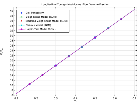
In the Settings window for 1D Plot Group, type Longitudinal Young's Modulus vs. Fiber Volume Fraction in the Label text field.
3
Locate the Data section. From the Dataset list, choose Cell Periodicity Study for Elastic Properties/Solution 2 (solidcp1solp).
4
From the Parameter selection (Load case) list, choose First.
5
Click to expand the Title section. From the Title type list, choose Manual.
6
In the Title text area, type Longitudinal Young's Modulus vs. Fiber Volume Fraction.
7
Locate the Plot Settings section.
8
Select the x-axis label checkbox. In the associated text field, type v<sub>f</sub>.
9
Select the y-axis label checkbox. In the associated text field, type E<sub>1</sub>/E<sub>m</sub>.
10
Locate the Legend section. From the Position list, choose Upper left.
Global 1
1
Right-click Longitudinal Young’s Modulus vs. Fiber Volume Fraction and choose Global.
2
In the Settings window for Global, locate the y-Axis Data section.
3
4
Locate the x-Axis Data section. From the Axis source data list, choose v_f.
5
Click to expand the Coloring and Style section. Find the Line markers subsection. From the Marker list, choose Cycle.
6
From the Positioning list, choose Interpolated.
7
Click to expand the Legends section. From the Legends list, choose Manual.
8
Duplicate or add this plot group twice in order to plot the remaining elastic properties. Use appropriate labels, titles, and expressions.
Longitudinal Coefficient of Thermal Expansion vs. Fiber Volume Fraction
1
In the Results toolbar, click  1D Plot Group.
2
In the Settings window for 1D Plot Group, locate the Data section.
3
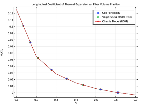
From the Dataset list, choose Cell Periodicity Study for Thermal Properties/Parametric Solutions 1 (sol9).
4
From the Parameter selection (para) list, choose From list.
5
In the Parameter values (para) list box, select 0.
6
In the Label text field, type Longitudinal Coefficient of Thermal Expansion vs. Fiber Volume Fraction.
7
Locate the Title section. From the Title type list, choose Manual.
8
In the Title text area, type Longitudinal Coefficient of Thermal Expansion vs. Fiber Volume Fraction.
9
Locate the Plot Settings section.
10
Select the x-axis label checkbox. In the associated text field, type v<sub>f</sub>.
11
Select the y-axis label checkbox. In the associated text field, type \alpha<sub>1</sub>/\alpha<sub>m</sub>.
Global 1
1
Right-click Longitudinal Coefficient of Thermal Expansion vs. Fiber Volume Fraction and choose Global.
2
In the Settings window for Global, click Replace Expression in the upper-right corner of the y-Axis Data section. From the menu, choose Component 1 (comp1) > Solid Mechanics > Cell periodicity > Coefficient of thermal expansion (material and geometry frames) - 1/K > solid.cp2.alphaXX - Coefficient of thermal expansion, XX-component.
3
Locate the y-Axis Data section. In the table, enter the following settings:
4
Locate the Coloring and Style section. Find the Line markers subsection. From the Marker list, choose Cycle.
5
From the Positioning list, choose Interpolated.
6
Locate the Legends section. From the Legends list, choose Manual.
7
8
In the Longitudinal Coefficient of Thermal Expansion vs. Fiber Volume Fraction toolbar, click  Plot.
Finally, group the plots for better readability.
In-plane Shear Modulus vs. Fiber Volume Fraction, Longitudinal Young’s Modulus vs. Fiber Volume Fraction, Transverse Young’s Modulus vs. Fiber Volume Fraction
1
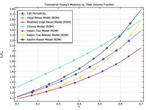
In the Model Builder window, under Results, Ctrl-click to select Longitudinal Young’s Modulus vs. Fiber Volume Fraction, Transverse Young’s Modulus vs. Fiber Volume Fraction, and In-plane Shear Modulus vs. Fiber Volume Fraction.
2
Elastic Properties
In the Settings window for Group, type Elastic Properties in the Label text field.
Longitudinal Coefficient of Thermal Expansion vs. Fiber Volume Fraction, Transverse Coefficient of Thermal Expansion vs. Fiber Volume Fraction
1
In the Model Builder window, under Results, Ctrl-click to select Longitudinal Coefficient of Thermal Expansion vs. Fiber Volume Fraction and Transverse Coefficient of Thermal Expansion vs. Fiber Volume Fraction.
2
Thermal Expansion Properties, Zero Poisson’s Ratio
In the Settings window for Group, type Thermal Expansion Properties, Zero Poisson's Ratio in the Label text field.
Longitudinal Coefficient of Thermal Expansion vs. Fiber Volume Fraction with Nonzero Poisson’s Ratio, Transverse Coefficient of Thermal Expansion vs. Fiber Volume Fraction with Nonzero Poisson’s Ratio
1
In the Model Builder window, under Results, Ctrl-click to select Longitudinal Coefficient of Thermal Expansion vs. Fiber Volume Fraction with Nonzero Poisson’s Ratio and Transverse Coefficient of Thermal Expansion vs. Fiber Volume Fraction with Nonzero Poisson’s Ratio.
2
Thermal Expansion Properties, Nonzero Poisson’s Ratio
In the Settings window for Group, type Thermal Expansion Properties, Nonzero Poisson's Ratio in the Label text field.