
|
|
|

|
C11
|
|||
|
C12
|
|||
|
C22
|
|||
|
C33
|

|
1
|
|
2
|
|
3
|
Click Add.
|
|
4
|
Click
|
|
5
|
|
6
|
Click
|
|
1
|
|
2
|
|
3
|
|
4
|
Browse to the model’s Application Libraries folder and double-click the file membrane_torsion_parameters.txt.
|
|
1
|
|
2
|
|
3
|
|
4
|
Browse to the model’s Application Libraries folder and double-click the file membrane_torsion_isotropic_properties.txt.
|
|
1
|
|
2
|
In the Settings window for Parameters, type Orthotropic Material Properties in the Label text field.
|
|
3
|
|
4
|
Browse to the model’s Application Libraries folder and double-click the file membrane_torsion_orthotropic_properties.txt.
|
|
1
|
|
2
|
|
1
|
|
2
|
|
3
|
Click
|
|
4
|
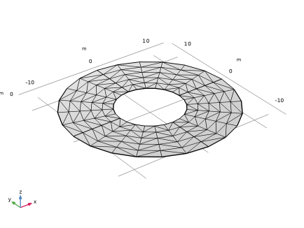
Browse to the model’s Application Libraries folder and double-click the file membrane_torsion_tria_mesh1.mphbin.
|
|
5
|
Click
|
|
1
|
|
2
|
|
3
|
|
1
|
|
2
|
Click
|
|
3
|
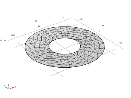
Browse to the model’s Application Libraries folder and double-click the file membrane_torsion_tria_mesh2.mphbin.
|
|
4
|
Click
|
|
1
|
|
2
|
|
1
|
|
2
|
|
3
|
Click
|
|
4
|
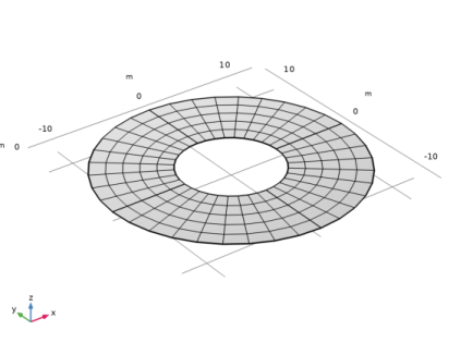
Browse to the model’s Application Libraries folder and double-click the file membrane_torsion_quad_mesh1.mphbin.
|
|
5
|
Click
|
|
1
|
|
2
|
|
1
|
|
2
|
|
3
|
Click
|
|
4
|
Browse to the model’s Application Libraries folder and double-click the file membrane_torsion_quad_mesh2.mphbin.
|
|
5
|
Click
|
|
1
|
|
2
|
|
3
|
|
1
|
In the Model Builder window, under Component 1 (comp1) > Membrane (mbrn) click Linear Elastic Material 1.
|
|
2
|
|
3
|
|
1
|
|
2
|
|
3
|
|
1
|
In the Model Builder window, under Component 1 (comp1) > Membrane (mbrn) click Thickness and Offset 1.
|
|
2
|
|
3
|
|
1
|
|
1
|
|
3
|
|
4
|
|
5
|
|
6
|
|
7
|
|
8
|
|
9
|
|
1
|
|
2
|
|
3
|
In the Show More Options dialog, in the tree, select the checkbox for the node Physics > Advanced Physics Options.
|
|
4
|
Click OK.
|
|
1
|
|
2
|
|
3
|
|
4
|
|
1
|
|
2
|
|
3
|
Locate the Material Contents section. In the table, enter the following settings:
|
|
1
|
|
2
|
|
3
|
Locate the Material Contents section. In the table, enter the following settings:
|
|
1
|
|
2
|
In the Settings window for Study, type Study: Three Noded Triangular (Pattern 1) in the Label text field.
|
|
3
|
|
1
|
|
2
|
|
3
|
Click
|
|
1
|
|
2
|
|
3
|
Select the Auxiliary sweep checkbox.
|
|
4
|
Click
|
|
1
|
|
2
|
|
3
|
In the Model Builder window, expand the Study: Three Noded Triangular (Pattern 1) > Solver Configurations > Solution 1 (sol1) > Stationary Solver 1 node, then click Parametric 1.
|
|
4
|
|
5
|
|
6
|
In the Model Builder window, under Study: Three Noded Triangular (Pattern 1) > Solver Configurations > Solution 1 (sol1) > Stationary Solver 1 click Fully Coupled 1.
|
|
7
|
|
8
|
|
9
|
|
10
|
|
11
|
|
1
|
|
2
|
Go to the Add Study window.
|
|
3
|
|
4
|
Click the Add Study button in the window toolbar.
|
|
5
|
|
1
|
In the Settings window for Study, type Study: Three Noded Triangular (Pattern 2) in the Label text field.
|
|
2
|
|
1
|
|
2
|
|
3
|
Click
|
|
1
|
|
2
|
|
4
|
|
5
|
Click
|
|
7
|
|
1
|
|
2
|
Go to the Add Study window.
|
|
3
|
|
4
|
Click the Add Study button in the window toolbar.
|
|
5
|
|
1
|
In the Settings window for Study, type Study: Four Noded Quadrilateral (Pattern 3) in the Label text field.
|
|
2
|
|
1
|
|
2
|
|
3
|
Click
|
|
1
|
|
2
|
|
4
|
|
5
|
Click
|
|
7
|
|
1
|
|
2
|
Go to the Add Study window.
|
|
3
|
|
4
|
Click the Add Study button in the window toolbar.
|
|
5
|
|
1
|
In the Settings window for Study, type Study: Nine Noded Quadrilateral (Pattern 4) in the Label text field.
|
|
2
|
|
1
|
|
2
|
|
3
|
Click
|
|
1
|
|
2
|
|
3
|
Select the Modify model configuration for study step checkbox.
|
|
4
|
|
5
|
|
6
|
Locate the Mesh Selection section. In the table, enter the following settings:
|
|
7
|
|
8
|
Click
|
|
10
|
|
1
|
|
2
|
|
3
|
Locate the Data section. From the Dataset list, choose Study: Three Noded Triangular (Pattern 1)/Parametric Solutions 1 (sol2).
|
|
4
|
|
5
|
|
6
|
|
1
|
|
2
|
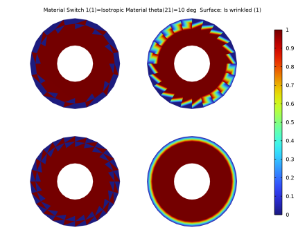
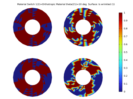
In the Settings window for Surface, click Replace Expression in the upper-right corner of the Expression section. From the menu, choose Component 1 (comp1) > Membrane > Wrinkling > mbrn.iswrinkled - Is wrinkled - 1.
|
|
3
|
|
4
|
|
5
|
|
6
|
|
7
|
|
1
|
|
2
|
|
3
|
From the Dataset list, choose Study: Three Noded Triangular (Pattern 2)/Parametric Solutions 2 (sol6).
|
|
4
|
|
5
|
|
6
|
|
7
|
|
1
|
|
2
|
|
3
|
From the Dataset list, choose Study: Four Noded Quadrilateral (Pattern 3)/Parametric Solutions 3 (sol10).
|
|
4
|
|
5
|
|
1
|
|
2
|
|
3
|
From the Dataset list, choose Study: Nine Noded Quadrilateral (Pattern 4)/Parametric Solutions 4 (sol14).
|
|
4
|
|
1
|
|
2
|
|
3
|
|
4
|
|
5
|
|
6
|
|
7
|
|
1
|
|
2
|
|
3
|
Click
|
|
4
|
|
5
|
|
6
|
Click OK.
|
|
7
|
|
9
|
Click
|
|
1
|
|
2
|
|
3
|
Click to expand the Window Settings section. Locate the Color Legend section. From the Position list, choose Right double.
|
|
1
|
|
2
|
|
3
|
|
4
|
|
1
|
|
2
|
|
3
|
|
4
|
|
5
|
|
1
|
|
2
|
|
3
|
|
4
|
|
5
|
|
1
|
|
2
|
|
3
|
|
4
|
|
5
|
|
1
|
|
2
|
|
3
|
Select the Show maximum and minimum values checkbox.
|
|
4
|
|
1
|
|
2
|
|
1
|
|
2
|
|
3
|
|
1
|
|
2
|
|
3
|
|
1
|
|
2
|
|
3
|
|
1
|
|
2
|
|
3
|
|
4
|
|
1
|
|
2
|
In the Settings window for Evaluation Group, type Maximum Wrinkling Measure (Isotropic) in the Label text field.
|
|
3
|
Locate the Data section. From the Dataset list, choose Study: Three Noded Triangular (Pattern 1)/Parametric Solutions 1 (sol2).
|
|
4
|
|
5
|
|
1
|
|
2
|
|
3
|
|
4
|
Click Replace Expression in the upper-right corner of the Expressions section. From the menu, choose Component 1 (comp1) > Membrane > Wrinkling > mbrn.lemm1.wr1.Beta - Wrinkling measure, material frame - 1.
|
|
1
|
|
2
|
|
3
|
From the Dataset list, choose Study: Three Noded Triangular (Pattern 2)/Parametric Solutions 2 (sol6).
|
|
4
|
|
5
|
|
1
|
|
2
|
|
3
|
From the Dataset list, choose Study: Four Noded Quadrilateral (Pattern 3)/Parametric Solutions 3 (sol10).
|
|
1
|
|
2
|
|
3
|
From the Dataset list, choose Study: Nine Noded Quadrilateral (Pattern 4)/Parametric Solutions 4 (sol14).
|
|
1
|
|
2
|
|
3
|
Select the Transpose checkbox.
|
|
4
|
|
1
|
In the Model Builder window, under Results, Ctrl-click to select Wrinkled Region, First Principal Stress, and Second Principal Stress.
|
|
2
|
Right-click and choose Group.
|
|
1
|
|
2
|
|
1
|
|
2
|
|
3
|
|
1
|
|
2
|
|
3
|
|
1
|
|
2
|
|
3
|
|
1
|
|
2
|
|
3
|
|
4
|
|
1
|
|
2
|
|
3
|
|
1
|
|
2
|
|
3
|
|
1
|
|
2
|
|
3
|
|
1
|
|
2
|
|
3
|
|
4
|
|
1
|
|
2
|
|
3
|
|
1
|
|
2
|
|
3
|
|
1
|
|
2
|
|
3
|
|
1
|
|
2
|
|
3
|
|
4
|
|
1
|
In the Model Builder window, right-click Maximum Wrinkling Measure (Isotropic) and choose Duplicate.
|
|
2
|
In the Settings window for Evaluation Group, type Maximum Wrinkling Measure (Orthotropic) in the Label text field.
|
|
3
|
|
1
|
In the Model Builder window, expand the Maximum Wrinkling Measure (Orthotropic) node, then click Surface Maximum 2.
|
|
2
|
|
3
|
|
1
|
|
2
|
|
3
|
|
1
|
|
2
|
|
3
|
|
4
|