PDF

Nonlinear Ferromagnetic Diaphragm
Introduction
A magnetic diaphragm is a flexible, thin structure that interacts with magnetic fields to perform mechanical or sensing functions. When subjected to an external magnetic field, the diaphragm deforms due to magnetomechanical interactions, converting magnetic energy into mechanical displacement or, conversely, mechanical deformation into changes in the magnetic field distribution. In this model, you will study the magnetomechanics of a magnetic diaphragm using the Magnetomechanics, Shell multiphysics interface. This interface combines the Shell and Magnetic Fields physics with moving mesh functionality, allowing simulation of the coupled mechanical deformation and magnetic field interactions for thin, flexible structures.
Model Definition
As shown in Figure 1, the model consists of two coupled parts: an electromagnet that generates a magnetic field when driven by a prescribed current input, and a thin elastic magnetic diaphragm driven by the magnetic field. The geometry is defined in an axisymmetric configuration, capturing the circular symmetry of the system. The model is geometrically similar to the one used in Ref. 1.
Figure 1: Model geometry definition. The axisymmetric model consists of an electromagnet and a magnetic diaphragm.
A radial pretension is also applied to the diaphragm, which will strongly affect its mechanical response to the magnetic loading. This setup allows for investigation of the magnetomechanical coupling between the electromagnetic field and the diaphragm. Such coupled models are relevant for the design of magnetically actuated thin structures, sensors, and vibration control devices.
The constitutive relation for the diaphragm material is nonlinear with the magnetization model given by Ref. 1:
.
Note that, in general, you can use other type of B-H relation. For details, see the AC/DC Module User’s Guide.
Results and Discussion
Figure 2 shows the displacement magnitude as a function of the input current for several pretension levels.
Figure 2: The displacement of the center of the diaphragm as a function of the current.
The blue curve on the top, which represents the case without pretension, shows an almost linear relationship between displacement and current and exhibits the largest displacement. As the pretension increases, the displacement decreases accordingly. This result demonstrates that the diaphragm becomes stiffer and more resistant to deformation when subjected to radial stretching, which is consistent with physical intuition.
Figure 3 shows the magnetic flux density on the diaphragm.
Figure 3: The z component of the magnetic flux density distribution on the diaphragm.
One can see that the magnetic flux density responds to the current input accordingly.
Initially, the applied current input is relatively weak, resulting in only small deformations of the magnetic diaphragm. This allows you to study the fundamental coupling between the electromagnetic and structural domains without introducing large nonlinear effects. To further explore the system behavior, you can increase the current input or modify the magnetic B–H curve. This provides valuable insight into how material properties and excitation levels influence both the stiffness and sensitivity of the diaphragm.
You can perform an additional study with the current increased to 4 A. Figure 4 shows the resulting geometry of the thin diaphragm. In this case, the diaphragm undergoes a large deformation and is strongly attracted to the magnet.
Figure 4: Magnetic flux density norm and field lines for a 4 A current. At this high current, the diaphragm is fully attracted to the magnet.
Reference
1. V.R. Jayaneththi, K.C. Aw, and A.J. McDaid, “Coupled magneto-mechanical modeling of non-linear ferromagnetic diaphragm systems,” Int. J. Mech. Sci., vol. 155, pp. 360–369, 2019.
Application Library path: Structural_Mechanics_Module/Magnetomechanics/magnetic_diaphragm
Modeling Instructions
From the File menu, choose New.
New
In the New window, click  Model Wizard.
Model Wizard
1
In the Model Wizard window, click  2D Axisymmetric.
2
In the Select Physics tree, select AC/DC > Electromagnetics and Mechanics > Magnetomechanics > Magnetomechanics, Shell.
3
Click Add.
4
Click  Study.
5
In the Select Study tree, select General Studies > Stationary.
6
Global Definitions
Parameters 1
1
In the Model Builder window, under Global Definitions click Parameters 1.
2
In the Settings window for Parameters, locate the Parameters section.
3
4
In the Model Builder window, click Parameters 1.
5
Geometry 1
Rectangle 1 (r1)
1
In the Geometry toolbar, click  Rectangle.
2
In the Settings window for Rectangle, locate the Size and Shape section.
3
In the Width text field, type EM1_r_outer.
4
In the Height text field, type EM1_height.
whole space
1
Right-click Rectangle 1 (r1) and choose Duplicate.
2
In the Settings window for Rectangle, type whole space in the Label text field.
3
Locate the Size and Shape section. In the Width text field, type EM1_r_outer*2.
4
In the Height text field, type EM1_height*1.5.
hollow area
1
Right-click whole space and choose Duplicate.
2
In the Settings window for Rectangle, type hollow area in the Label text field.
3
Locate the Size and Shape section. In the Width text field, type EM1_r_core.
4
In the Height text field, type EM1_hollow_height.
Rectangle 4 (r4)
1
In the Geometry toolbar, click  Rectangle.
2
In the Settings window for Rectangle, locate the Size and Shape section.
3
In the Width text field, type gray_area_width.
4
In the Height text field, type EM1_hollow_height.
5
Locate the Position section. In the r text field, type EM1_height*0.35.
6
In the z text field, type EM1_height-EM1_hollow_height.
Line Segment 1 (ls1)
1
In the Geometry toolbar, click  More Primitives and choose Line Segment.
2
In the Settings window for Line Segment, locate the Starting Point section.
3
From the Specify list, choose Coordinates.
4
In the z text field, type EM1_height+gap_distance.
5
Locate the Endpoint section. From the Specify list, choose Coordinates.
6
In the r text field, type diaphragm_r.
7
In the z text field, type EM1_height+gap_distance.
Rectangle 5 (r5)
1
In the Geometry toolbar, click  Rectangle.
2
In the Settings window for Rectangle, locate the Size and Shape section.
3
In the Width text field, type gray_area_width*0.9.
4
In the Height text field, type EM1_hollow_height*0.9.
5
Locate the Position section. In the r text field, type EM1_height*0.36.
6
In the z text field, type (EM1_height-EM1_hollow_height*0.95).
7
Click  Build All Objects.
8
Click the  Zoom Extents button in the Graphics toolbar.
Add Material
1
In the Materials toolbar, click  Add Material to open the Add Material window.
2
Go to the Add Material window.
3
In the tree, select Built-in > Copper.
4
Click the Add to Component button in the window toolbar.
Materials
Copper (mat1)
1
2
In the Settings window for Material, locate the Geometric Entity Selection section.
3
Click  Clear Selection.
4
Add Material
1
Go to the Add Material window.
2
In the Search text field, type Low Carbon Steel Soft Iron.
3
Click Search.
4
In the tree, select Nonlinear Magnetic > Low Carbon Steel > Low Carbon Steel Soft Iron.
5
Click the Add to Component button in the window toolbar.
Materials
Low Carbon Steel Soft Iron (mat2)
1
In the Model Builder window, expand the Component 1 (comp1) > Materials > Low Carbon Steel Soft Iron (mat2) node, then click Low Carbon Steel Soft Iron (mat2).
2
Magnetic polymer composites
1
In the Model Builder window, right-click Materials and choose Blank Material.
2
In the Settings window for Material, locate the Geometric Entity Selection section.
3
From the Geometric entity level list, choose Boundary.
4
5
In the Label text field, type Magnetic polymer composites.
6
Locate the Material Contents section. In the table, enter the following settings:
7
In the Model Builder window, expand the Component 1 (comp1) > Materials > Magnetic polymer composites (mat3) node.
Results
Global Evaluation Sweep 1
1
In the Model Builder window, expand the Results node.
2
Right-click Results > Derived Values and choose More Derived Values > Global Evaluation Sweep.
3
In the Settings window for Global Evaluation Sweep, locate the Parameters section.
4
5
Locate the Expressions section. In the table, enter the following settings:
6
Click  Evaluate.
Materials
Magnetic polymer composites (mat3)
1
In the Model Builder window, under Component 1 (comp1) > Materials click Magnetic polymer composites (mat3).
2
In the Settings window for Material, locate the Material Contents section.
3
Moving Mesh
Deforming Domain 1
1
In the Model Builder window, under Component 1 (comp1) > Moving Mesh click Deforming Domain 1.
2
Symmetry/Roller 1
1
In the Model Builder window, click Symmetry/Roller 1.
2
Magnetic Fields (mf)
Domain Coil 1
1
In the Physics toolbar, click  Domains and choose Domain Coil.
2
3
In the Settings window for Domain Coil, locate the Material Type section.
4
From the Material type list, choose Solid.
5
Locate the Coil section. From the Conductor model list, choose Homogenized multiturn.
6
In the Icoil text field, type current_I.
7
Locate the Homogenized Conductor section. In the N text field, type N_turn.
Ampère’s Law in Solids 1
1
In the Physics toolbar, click  Domains and choose Ampère’s Law in Solids.
2
Add Material
1
Go to the Add Material window.
2
In the Search text field, type epoxy resin.
3
Click Search.
4
In the tree, select Material Library > Epoxies, Adhesives, and Underfills > Filled epoxy resin (X238) > Filled epoxy resin (X238) [solid].
5
Click the Add to Component button in the window toolbar.
6
In the Materials toolbar, click  Add Material to close the Add Material window.
Materials
Filled epoxy resin (X238) [solid] (mat4)
1
2
In the Model Builder window, expand the Filled epoxy resin (X238) [solid] (mat4) node.
3
In the Model Builder window, expand the Component 1 (comp1) > Materials > Filled epoxy resin (X238) [solid] (mat4) > Basic (def) node, then click Filled epoxy resin (X238) [solid] (mat4).
4
In the Settings window for Material, locate the Material Contents section.
5
Magnetic Fields (mf)
Magnetic Shielding 1
1
In the Physics toolbar, click  Boundaries and choose Magnetic Shielding.
2
3
In the Settings window for Magnetic Shielding, locate the Magnetic Shielding section.
4
In the ds text field, type diaphragm_thickness.
Materials
Low Carbon Steel Soft Iron (mat2)
1
In the Model Builder window, under Component 1 (comp1) > Materials click Low Carbon Steel Soft Iron (mat2).
2
In the Settings window for Material, locate the Material Contents section.
3
As a first step, we assume that the magnetic diaphragm exhibits linear magnetic properties.
Magnetic Fields (mf)
Magnetic Shielding 1
1
In the Model Builder window, under Component 1 (comp1) > Magnetic Fields (mf) click Magnetic Shielding 1.
2
In the Settings window for Magnetic Shielding, locate the Magnetic Shielding section.
3
From the μr list, choose User defined. In the associated text field, type 100.
Shell (shell)
Thickness and Offset 1
1
In the Model Builder window, under Component 1 (comp1) > Shell (shell) click Thickness and Offset 1.
2
In the Settings window for Thickness and Offset, locate the Thickness and Offset section.
3
In the d0 text field, type diaphragm_thickness.
Prescribed Displacement/Rotation 1
1
In the Physics toolbar, click  Points and choose Prescribed Displacement/Rotation.
2
3
In the Settings window for Prescribed Displacement/Rotation, locate the Prescribed Displacement section.
4
From the Displacement in r direction list, choose Prescribed.
5
In the u0r text field, type pretension_disp.
6
From the Displacement in z direction list, choose Prescribed.
7
Locate the Prescribed Rotation section. From the By list, choose Rotation.
8
In the Model Builder window, click Shell (shell).
9
In the Settings window for Shell, locate the Boundary Selection section.
10
In the list box, select 1 (not applicable).
11
Click  Clear Selection.
12
Prescribed Displacement/Rotation 2
1
In the Physics toolbar, click  Boundaries and choose Prescribed Displacement/Rotation.
We assume that the diaphragm can undergo sufficiently large deformation to make contact with the magnet, though this is contingent on the magnitude of the applied current and the material properties.
2
3
In the Settings window for Prescribed Displacement/Rotation, locate the Prescribed Displacement section.
4
From the Displacement in z direction list, choose Limited.
5
In the u0z,min text field, type -gap_distance+diaphragm_thickness/2.
Multiphysics
Magnetomechanics, Boundary 1 (mmfb1)
1
In the Model Builder window, expand the Component 1 (comp1) > Multiphysics > Magnetomechanics, Boundary 1 (mmfb1) node, then click Magnetomechanics, Boundary 1 (mmfb1).
2
In the Settings window for Magnetomechanics, Boundary, locate the Boundary Selection section.
3
Click  Clear Selection.
4
Mesh 1
1
In the Model Builder window, under Component 1 (comp1) click Mesh 1.
2
In the Settings window for Mesh, locate the Physics-Controlled Mesh section.
3
From the Element size list, choose Extra fine.
4
Click  Build All.
Study 1
Parametric Sweep
1
In the Study toolbar, click  Parametric Sweep.
2
In the Settings window for Parametric Sweep, locate the Study Settings section.
3
4
Step 1: Stationary
1
In the Model Builder window, click Step 1: Stationary.
2
In the Settings window for Stationary, click to expand the Study Extensions section.
3
Select the Auxiliary sweep checkbox.
4
5
6
In the Study toolbar, click  Compute.
Results
Magnetic Flux Density (mf)
1
In the Settings window for 2D Plot Group, locate the Data section.
2
From the Parameter value (pretension_disp (m)) list, choose 0.
3
From the Parameter value (current_I (A)) list, choose 0.1.
4
In the Magnetic Flux Density (mf) toolbar, click  Plot.
At this point, the user may pause to experiment with different values for the input current (current_I) and the magnetic properties of the material. Next, we will introduce a B–H curve for the magnetic shielding.
Materials
Magnetic polymer composites (mat3)
1
In the Model Builder window, under Component 1 (comp1) > Materials click Magnetic polymer composites (mat3).
2
In the Settings window for Material, click to expand the Material Properties section.
3
In the Material properties tree, select Electromagnetic Models > B-H Curve.
4
Click  Add to Material.
5
In the Model Builder window, under Component 1 (comp1) > Materials > Magnetic polymer composites (mat3) click B-H curve (BHCurve).
6
In the Settings window for B-H Curve, locate the Output Properties section.
7
Interpolation 1 (int1)
1
Right-click Component 1 (comp1) > Materials > Magnetic polymer composites (mat3) > B-H curve (BHCurve) and choose Functions > Interpolation.
2
In the Settings window for Interpolation, locate the Definition section.
3
From the Data source list, choose Result table.
Results
Global Evaluation Sweep 1
1
In the Model Builder window, expand the Results > Tables node, then click Results > Derived Values > Global Evaluation Sweep 1.
2
In the Settings window for Global Evaluation Sweep, click  Evaluate.
3
Locate the Data section. From the Dataset list, choose Study 1/Solution 1 (sol1).
4
Click  Evaluate.
5
Clicknext to  Evaluate, then choose Table 1 - Global Evaluation Sweep 1.
Table 1
1
In the Model Builder window, under Results > Tables click Table 1.
2
In the Settings window for Table, click  Update.
Materials
Interpolation 1 (int1)
1
In the Model Builder window, under Component 1 (comp1) > Materials > Magnetic polymer composites (mat3) > B-H curve (BHCurve) click Interpolation 1 (int1).
2
In the Settings window for Interpolation, click to expand the Related Functions section.
3
Select the Define inverse function checkbox.
4
Select the Define primitive function checkbox.
5
Select the Define random function checkbox.
6
In the Inverse function name text field, type BH_inv.
7
In the Primitive function name text field, type BH_prim.
8
Clear the Define random function checkbox.
9
10
Locate the Data Column Settings section. In the table, click to select the cell at row number 1 and column number 2.
11
In the Unit text field, type A/m.
12
13
In the Unit text field, type T.
14
Magnetic polymer composites (mat3)
In the Model Builder window, expand the Component 1 (comp1) > Materials > Magnetic polymer composites (mat3) node.
Interpolation 1 (int1, BH_inv, BH_prim)
1
In the Model Builder window, expand the Component 1 (comp1) > Materials > Magnetic polymer composites (mat3) > B-H curve (BHCurve) node, then click Interpolation 1 (int1, BH_inv, BH_prim).
2
3
In the Name text field, type BH.
Magnetic Fields (mf)
Magnetic Shielding 1
1
In the Model Builder window, under Component 1 (comp1) > Magnetic Fields (mf) click Magnetic Shielding 1.
2
In the Settings window for Magnetic Shielding, locate the Magnetic Shielding section.
3
From the μr list, choose From material.
4
From the Magnetization model list, choose B-H curve.
5
In the Home toolbar, click  Compute.
Results
Displacement Magnitude
1
In the Results toolbar, click  1D Plot Group.
2
In the Settings window for 1D Plot Group, type Displacement Magnitude in the Label text field.
3
Locate the Data section. From the Dataset list, choose Study 1/Parametric Solutions 1 (sol2).
4
Click to expand the Title section. From the Title type list, choose Manual.
5
In the Title text area, type Displacement magnitude, midpoint.
6
Locate the Legend section. From the Position list, choose Upper left.
7
In the Displacement Magnitude toolbar, click  Plot.
Point Graph 1
1
Right-click Displacement Magnitude and choose Point Graph.
2
3
In the Settings window for Point Graph, locate the y-Axis Data section.
4
In the Expression text field, type shell.disp.
5
From the Unit list, choose mm.
6
In the Displacement Magnitude toolbar, click  Plot.
7
Click to expand the Legends section. Select the Show legends checkbox.
8
From the Legends list, choose Evaluated.
9
In the Legend text field, type Pretension displacement: eval(pretension_disp, mm) mm.
10
In the Displacement Magnitude toolbar, click  Plot.
Magnetic Flux Density on the Diaphragm
1
In the Results toolbar, click  1D Plot Group.
2
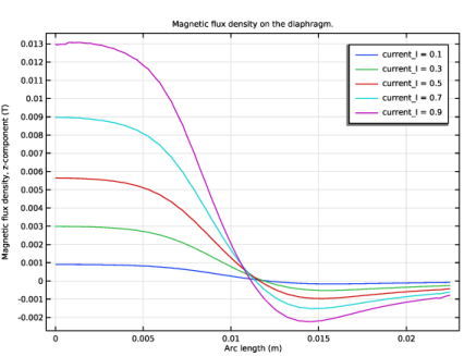
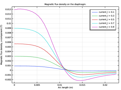
In the Settings window for 1D Plot Group, type Magnetic Flux Density on the Diaphragm in the Label text field.
3
Locate the Data section. From the Dataset list, choose Study 1/Parametric Solutions 1 (sol2).
4
From the Parameter selection (pretension_disp) list, choose First.
5
Locate the Title section. From the Title type list, choose Manual.
6
In the Title text area, type Magnetic flux density on the diaphragm..
Line Graph 1
1
Right-click Magnetic Flux Density on the Diaphragm and choose Line Graph.
2
3
In the Settings window for Line Graph, locate the y-Axis Data section.
4
In the Expression text field, type mf.Bz.
5
In the Magnetic Flux Density on the Diaphragm toolbar, click  Plot.
6
Click to expand the Legends section. From the Legends list, choose Evaluated.
7
Select the Show legends checkbox.
8
In the Legend text field, type current_I = eval(current_I).
Revolution 2D 1
In the Model Builder window, expand the Results > Datasets node, then click Revolution 2D 1.
Selection
1
In the Results toolbar, click  Attributes and choose Selection.
2
In the Settings window for Selection, locate the Geometric Entity Selection section.
3
From the Geometric entity level list, choose Domain.
4
Revolution 2D 2
Right-click Revolution 2D 1 and choose Duplicate.
Selection
1
In the Model Builder window, expand the Revolution 2D 2 node, then click Selection.
2
In the Settings window for Selection, locate the Geometric Entity Selection section.
3
From the Geometric entity level list, choose Boundary.
4
Revolution 2D 2
1
In the Model Builder window, click Revolution 2D 2.
2
In the Settings window for Revolution 2D, click to expand the Revolution Layers section.
3
Clear the Add end caps if the revolution is not full checkbox.
Arrow Surface 1
1
In the Model Builder window, expand the Results > Magnetic Flux Density, Revolved Geometry (mf) node.
2
Right-click Magnetic Flux Density, Revolved Geometry (mf) and choose Arrow Surface.
3
In the Settings window for Arrow Surface, locate the Data section.
4
From the Dataset list, choose Revolution 2D 2.
5
From the Solution parameters list, choose From parent.
6
Locate the Coloring and Style section. From the Color list, choose Black.
7
Locate the Arrow Positioning section. In the Number of arrows text field, type 40.
Surface 1
1
In the Model Builder window, right-click Magnetic Flux Density, Revolved Geometry (mf) and choose Surface.
2
Click the  Show Grid button in the Graphics toolbar.
3
In the Settings window for Surface, locate the Data section.
4
From the Dataset list, choose Revolution 2D 2.
5
From the Solution parameters list, choose From parent.
6
In the Magnetic Flux Density, Revolved Geometry (mf) toolbar, click  Plot.
7
Click to expand the Inherit Style section. From the Plot list, choose Volume 1.
8
In the Magnetic Flux Density, Revolved Geometry (mf) toolbar, click  Plot.
9
Click the  Transparency button in the Graphics toolbar.
10
From the Plot list, choose Contour 1.
11
In the Magnetic Flux Density, Revolved Geometry (mf) toolbar, click  Plot.
Magnetic Flux Density, Revolved Geometry (mf)
1
In the Model Builder window, click Magnetic Flux Density, Revolved Geometry (mf).
2
In the Settings window for 3D Plot Group, locate the Data section.
3
From the Parameter value (pretension_disp (m)) list, choose 7.5E-4.
4
Click to expand the Title section. From the Title type list, choose Manual.
5
In the Title text area, type Magnetic flux density (T).
6
Clear the Parameter indicator text field.
7
In the Magnetic Flux Density, Revolved Geometry (mf) toolbar, click  Plot.
8
Click  Plot First.
9
Click  Plot Last.
Next, we visually examine the mesh under different current inputs.
Moving Mesh
1
In the Model Builder window, click Moving Mesh.
2
In the Settings window for 2D Plot Group, locate the Data section.
3
From the Parameter value (pretension_disp (m)) list, choose 0.
4
In the Moving Mesh toolbar, click  Plot.
5
Click  Plot First.
6
Click  Plot Last.
Stress, 3D (shell)
1
In the Model Builder window, click Stress, 3D (shell).
2
In the Settings window for 3D Plot Group, locate the Data section.
3
From the Parameter value (pretension_disp (m)) list, choose 0.
4
In the Stress, 3D (shell) toolbar, click  Plot.
Once comfortable with this basic model, more advanced effects—such as nonlinear magnetization and material anisotropy—can be incorporated to achieve a more accurate and comprehensive simulation. It is strongly recommended that the user experiment with different input currents and materials with varying mechanical properties to explore their effects on the diaphragm’s behavior.
Add Study
1
In the Home toolbar, click  Add Study to open the Add Study window.
2
Go to the Add Study window.
3
Find the Studies subsection. In the Select Study tree, select General Studies > Stationary.
4
Click the Add Study button in the window toolbar.
5
In the Home toolbar, click  Add Study to close the Add Study window.
Global Definitions
Parameters 1
1
In the Settings window for Parameters, locate the Parameters section.
2
3
In the Home toolbar, click  Compute.
Results
Revolution 2D 3
In the Model Builder window, under Results > Datasets click Revolution 2D 3.
Selection
1
In the Results toolbar, click  Attributes and choose Selection.
2
In the Settings window for Selection, locate the Geometric Entity Selection section.
3
From the Geometric entity level list, choose Domain.
4
Revolution 2D 4
In the Model Builder window, under Results > Datasets click Revolution 2D 4.
Selection
1
In the Results toolbar, click  Attributes and choose Selection.
2
In the Settings window for Selection, locate the Geometric Entity Selection section.
3
From the Geometric entity level list, choose Boundary.
4
Arrow Surface 1
1
In the Model Builder window, expand the Results > Magnetic Flux Density, Revolved Geometry (mf) 1 node.
2
Right-click Results > Magnetic Flux Density, Revolved Geometry (mf) > Arrow Surface 1 and choose Copy.
Magnetic Flux Density, Revolved Geometry (mf) 1
1
In the Model Builder window, under Results click Magnetic Flux Density, Revolved Geometry (mf) 1.
2
In the Settings window for 3D Plot Group, locate the Title section.
3
From the Title type list, choose Manual.
4
In the Magnetic Flux Density, Revolved Geometry (mf) 1 toolbar, click  Plot.
Arrow Surface 1
Right-click Magnetic Flux Density, Revolved Geometry (mf) 1 and choose Paste Arrow Surface.
Surface 1
In the Model Builder window, under Results > Magnetic Flux Density, Revolved Geometry (mf) right-click Surface 1 and choose Copy.
Surface 1
In the Model Builder window, right-click Magnetic Flux Density, Revolved Geometry (mf) 1 and choose Paste Surface.
Arrow Surface 1
1
In the Settings window for Arrow Surface, locate the Coloring and Style section.
2
Volume 1
1
In the Model Builder window, click Volume 1.
2
In the Settings window for Volume, locate the Coloring and Style section.
3
Set the Color calibration parameter value to -1.5.
Arrow Surface 1
1
In the Model Builder window, click Arrow Surface 1.
2
In the Settings window for Arrow Surface, locate the Data section.
3
From the Dataset list, choose Revolution 2D 4.
4
In the Magnetic Flux Density, Revolved Geometry (mf) 1 toolbar, click  Plot.
5
Locate the Coloring and Style section. In the Scale factor text field, type 0.08.
6
Locate the Arrow Positioning section. In the Number of arrows text field, type 150.
7
In the Magnetic Flux Density, Revolved Geometry (mf) 1 toolbar, click  Plot.
Surface 1
1
In the Model Builder window, click Surface 1.
2
In the Settings window for Surface, locate the Data section.
3
From the Dataset list, choose Revolution 2D 4.
4
Locate the Inherit Style section. From the Plot list, choose Arrow Surface 1.
5
Locate the Coloring and Style section. From the Color table list, choose HeatCamera.
6
From the Color table transformation list, choose Nonlinear.
7
Set the Color calibration parameter value to -1.5.
8
In the Magnetic Flux Density, Revolved Geometry (mf) 1 toolbar, click  Plot.
9
Click the  Show Grid button in the Graphics toolbar.
10
Click the  Zoom Extents button in the Graphics toolbar.