PDF

In-Plane Framework with Discrete Mass and Mass Moment of Inertia
Introduction
In the following example you build and solve a 2D beam model using the 2D Structural Mechanics Beam interface. This example describes the eigenfrequency analysis of a simple geometry. A point mass and point mass moment of inertia are used. The two first eigenfrequencies are compared with the values given by an analytical expression.
In addition, it is shown how to evaluate modal participation factors and modal masses.
Model Definition
The geometry consists of a frame with one horizontal and one vertical member. The cross section of both members has an area, A, and an area moment of inertia, I. The length of each member is L and Young’s modulus is E. A point mass m is added at the middle of the horizontal member and a point mass moment of inertia J at the corner (see Figure 1 below).
Figure 1: Definition of the problem.
GEOMETRY
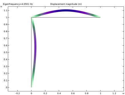
The framework members has a square cross section with a side length of 0.03 m giving an area of A = 9·104 m2 and an area moment of inertia of  I = 0.034/12 m4.
Material
Young’s modulus E = 200 GPa.
Mass
Point mass m = 1000 kg.
Point mass moment of inertia J = m r2 where r is chosen as L/4. This gives the value 62.5 kgm2.
Constraints
The beam is pinned at x = 0, y = 0 and x = 1, y = 1, meaning that the displacements are constrained whereas the rotational degrees of freedom are free.
Results and Discussion
The analytical values for the two first eigenfrequencies fe1 and fe2 are given by:
and
where ω is the angular frequency.
The following table shows a comparison between the eigenfrequencies calculated with COMSOL Multiphysics and the analytical values.
The following two plots visualize the two eigenmodes.
Figure 2: The first eigenmode.
Figure 3: The second eigenmode.
Because the beams have no density in this example, the total mass is the 1000 kg supplied by the point mass. The mass moment of inertia is also a point contribution, and has the value 62.5 kgm2. The mass represented by the computed eigenmodes can be evaluated using the modal participation factors, see Figure 4 and Figure 5. In this case, it can be seen that in the y direction, the correspondence is perfect, while almost none of the mass in the x direction is represented. The axial deformation mode for the horizontal member has a higher frequency, and was not computed. Similarly, all rotational inertia is captured by the first two modes.
Figure 4: Participation factors for each eigenfrequency.
Figure 5: Summed modal masses.
Notes About the COMSOL Implementation
The variables for evaluation of participation factors are created in the Participation Factors node under Definitions. This node is created automatically when an Eigenfrequency study is added.
Application Library path: Structural_Mechanics_Module/Verification_Examples/inplane_framework_freq
Modeling Instructions
From the File menu, choose New.
New
In the New window, click  Model Wizard.
Model Wizard
1
In the Model Wizard window, click  2D.
2
In the Select Physics tree, select Structural Mechanics > Beam (beam).
3
Click Add.
4
Click  Study.
5
In the Select Study tree, select General Studies > Eigenfrequency.
6
Global Definitions
Parameters 1
1
In the Model Builder window, under Global Definitions click Parameters 1.
2
In the Settings window for Parameters, locate the Parameters section.
3
Click  Load from File.
4
Geometry 1
Polygon 1 (pol1)
1
In the Geometry toolbar, click  Polygon.
2
In the Settings window for Polygon, locate the Object Type section.
3
From the Type list, choose Open curve.
4
Locate the Coordinates section. In the table, enter the following settings:
5
Click  Build All Objects.
Materials
Material 1 (mat1)
1
In the Model Builder window, under Component 1 (comp1) right-click Materials and choose Blank Material.
2
In the Settings window for Material, locate the Material Contents section.
3
Beam (beam)
Cross-Section Data 1
1
In the Model Builder window, under Component 1 (comp1) > Beam (beam) click Cross-Section Data 1.
2
In the Settings window for Cross-Section Data, locate the Cross-Section Definition section.
3
From the Section type list, choose Rectangle.
4
In the hy text field, type a.
5
In the hz text field, type a.
Pinned 1
1
In the Physics toolbar, click  Points and choose Pinned.
2
Point Mass 1
1
In the Physics toolbar, click  Points and choose Point Mass.
2
3
In the Settings window for Point Mass, locate the Point Mass section.
4
In the m text field, type m.
Point Mass 2
1
In the Physics toolbar, click  Points and choose Point Mass.
2
3
In the Settings window for Point Mass, locate the Point Mass section.
4
In the Jz text field, type J.
Study 1
Step 1: Eigenfrequency
1
In the Model Builder window, under Study 1 click Step 1: Eigenfrequency.
2
In the Settings window for Eigenfrequency, locate the Study Settings section.
3
Select the Desired number of eigenfrequencies checkbox. In the associated text field, type 2.
4
In the Study toolbar, click  Compute.
Results
Line 1
1
In the Model Builder window, expand the Results > Mode Shape (beam) node, then click Line 1.
2
In the Mode Shape (beam) toolbar, click  Plot.
3
Click the  Zoom Extents button in the Graphics toolbar.
Mode Shape (beam)
1
In the Model Builder window, click Mode Shape (beam).
2
In the Settings window for 2D Plot Group, locate the Data section.
3
From the Eigenfrequency (Hz) list, choose 8.6474.
4
In the Mode Shape (beam) toolbar, click  Plot.
Compare the computed eigenfrequencies to the analytical values.
Eigenfrequency Comparison
1
In the Results toolbar, click  Global Evaluation.
2
In the Settings window for Global Evaluation, type Eigenfrequency Comparison in the Label text field.
3
Locate the Expressions section. In the table, enter the following settings:
4
Click  Evaluate.
Participation Factors (Study 1)
1
In the Model Builder window, under Results click Participation Factors (Study 1).
2
In the Participation Factors (Study 1) toolbar, click  Evaluate.
Examine the modal participation factors.
Finally, compute the total effective mass accounted for in the computed eigenmodes.
Summed Modal Masses
1
In the Results toolbar, click  Global Evaluation.
2
In the Settings window for Global Evaluation, type Summed Modal Masses in the Label text field.
3
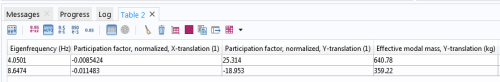
Click Replace Expression in the upper-right corner of the Expressions section. From the menu, choose Component 1 (comp1) > Definitions > Participation Factors 1 > Effective modal mass > mpf1.mEffLY - Effective modal mass, Y-translation - kg.
4
Locate the Expressions section. In the table, enter the following settings:
5
Locate the Data Series Operation section. From the Transformation list, choose Integral.
6
From the Method list, choose Summation.
7
Click  Evaluate.