PDF

Vibrations of an Impeller
Introduction
This tutorial model demonstrates the use of dynamic cyclic symmetry with postprocessing on the full geometry. A 3D impeller with eight identical blades can be divided into eight sectors of symmetry. The model computes the fundamental frequencies for the full impeller geometry and compares them to the values computed for a single sector with the cyclic symmetry boundary conditions applied on two sector boundaries. It also demonstrates how to set up a frequency response analysis for one sector of symmetry, and how to postprocess the results into the full geometry by using the sector datasets. The results for one sector are in very good agreement with the computations on the full geometry, while both the computational time and memory requirements are significantly reduced.
Model Definition
Figure 1 shows the impeller geometry. The problem is solved using the Cartesian coordinate system in 3D.
Figure 1: Impeller geometry.
The geometry can be divided into eight identical parts, each represented by a sector with an angle θ = π/4 with respect to rotation around the z-axis; see Figure 2.
Figure 2: Sector of periodicity.
The impeller is made of aluminum, and is supposed to be mounted on a shaft. The mounting boundary is modeled via a fixed constraint, and all possible effects of the shaft rotation are neglected.
The analysis is based on the Floquet theory which can be applied to the problem of small-amplitude vibrations of spatially periodic structures, Ref. 1. This includes the case of cyclic symmetry studied in this example.
For an eigenfrequency study, one can show that all the eigenmodes of the full problem can be found by performing the analysis on one sector of symmetry only and imposing the cyclic symmetry of the eigenmodes with an angle of periodicity , where the cyclic symmetry mode number m can vary from 0 to N/2, with N being the total number of sectors so that θ = 2π/N.
Results and Discussion
In the first part of the analysis, you perform an eigenfrequency analysis of a single sector of periodicity, and then of the full geometry. A sweep over all required values of the cyclic symmetry parameter recovers all the eigenfrequencies of the full model with decent accuracy. See the Modeling Instructions section for in-detail comparison of the results and discussion of the performance gains.
In the second part, you perform a frequency-response analysis. Again, first of the sector of periodicity, and then of the full impeller geometry. The excitation is a pressure load applied to all free boundaries of the impeller. You enter it as a normal component of the boundary load using the expression
using the magnitude of p0 = 104 Pa and cyclic symmetry parameter m = 3. The excitation frequency is 200 Hz. Figure 3 and Figure 4 show very good agreement between the results computed on the full and reduced geometry.
Figure 3: Frequency response computed on the sector of periodicity only, and then visualized over the full geometry.
Figure 4: Frequency response computed for the full geometry.
Notes About the COMSOL Implementation
Meshing
You use an unstructured mesh with the same size of the mesh elements for both calculations on one sector of symmetry and on the full geometry, see Figure 5. This helps to compare the results for this tutorial model. In practice, the mesh used for computations on the sector could be much finer, so that the results obtained via such geometry reduction would provide significantly better resolution of the results under the same memory requirements as for the full geometry (with a coarser mesh).
Figure 5: Meshed geometry.
Cyclic SYMMETRY conditions and Postprocessing
To set up the cyclic symmetry conditions, you use the predefined functionality available in COMSOL Multiphysics within the Solid Mechanics interface under the Periodic Condition boundary feature. This imposes the proper boundary coupling condition on the sector boundaries.
You visualize the results computed for one sector over the full geometry by making use of the predefined type of derived dataset called Sector 3D, which is available under the Results node in the COMSOL Desktop.
Reference
1. B. Lalanne and M. Touratier, “Aeroelastic Vibrations and Stability in Cyclic Symmetric Domains,” Int. J. Rotating Machinery, vol. 6, no. 6, pp. 445–452, 2000.
Application Library path: Structural_Mechanics_Module/Dynamics_and_Vibration/impeller
Modeling Instructions
From the File menu, choose New.
New
In the New window, click  Model Wizard.
Model Wizard
1
In the Model Wizard window, click  3D.
2
In the Select Physics tree, select Structural Mechanics > Solid Mechanics (solid).
3
Click Add.
4
Click  Study.
5
In the Select Study tree, select General Studies > Eigenfrequency.
6
Geometry 1
Import the prebuilt geometry for the impeller from a file.
Import 1 (imp1)
1
In the Geometry toolbar, click  Import.
2
In the Settings window for Import, locate the Source section.
3
Click  Browse.
4
5
Click  Import.
6
In the Geometry toolbar, click  Build All.
7
Click the  Go to Default View button in the Graphics toolbar.
8
Click the  Go to XY View button in the Graphics toolbar.
The complete geometry should look similar to that shown in Figure 1 and Figure 2.
Now create selections to easily apply loads and boundary conditions.
Definitions
Constrained Boundaries
1
In the Definitions toolbar, click  Explicit.
2
In the Settings window for Explicit, locate the Input Entities section.
3
From the Geometric entity level list, choose Boundary.
4
5
Select the Group by continuous tangent checkbox.
6
In the Label text field, type Constrained Boundaries.
Explicit 2
1
In the Definitions toolbar, click  Explicit.
2
In the Settings window for Explicit, locate the Input Entities section.
3
From the Geometric entity level list, choose Boundary.
4
5
Select the Group by continuous tangent checkbox.
Tip
1
In the Definitions toolbar, click  Explicit.
2
In the Settings window for Explicit, locate the Input Entities section.
3
From the Geometric entity level list, choose Boundary.
4
In the Label text field, type Tip.
5
Load Boundaries
1
In the Definitions toolbar, click  Union.
2
In the Settings window for Union, locate the Geometric Entity Level section.
3
From the Level list, choose Boundary.
4
Locate the Input Entities section. Under Selections to add, click  Add.
5
In the Add dialog, in the Selections to add list, choose Explicit 2 and Tip.
6
7
In the Settings window for Union, type Load Boundaries in the Label text field.
8
Click in the Graphics window and then press Ctrl+A to select all boundaries.
Free Boundaries
1
In the Definitions toolbar, click  Complement.
2
In the Settings window for Complement, locate the Geometric Entity Level section.
3
From the Level list, choose Boundary.
4
Locate the Input Entities section. Under Selections to invert, click  Add.
5
In the Add dialog, select Constrained Boundaries in the Selections to invert list.
6
7
In the Settings window for Complement, type Free Boundaries in the Label text field.
Global Definitions
Parameters 1
1
In the Model Builder window, under Global Definitions click Parameters 1.
2
In the Settings window for Parameters, locate the Parameters section.
3
Solid Mechanics (Full)
1
In the Model Builder window, under Component 1 (comp1) click Solid Mechanics (solid).
2
In the Settings window for Solid Mechanics, type Solid Mechanics (Full) in the Label text field.
Component 1 (comp1)
Add a second Solid Mechanics interface to use for the computations on the reduced geometry only.
Add Physics
1
In the Home toolbar, click  Add Physics to open the Add Physics window.
2
Go to the Add Physics window.
3
In the tree, select Structural Mechanics > Solid Mechanics (solid).
4
Click the Add to Component 1 button in the window toolbar.
5
In the Home toolbar, click  Add Physics to close the Add Physics window.
Solid Mechanics (Sector)
1
2
In the Settings window for Solid Mechanics, type Solid Mechanics (Sector) in the Label text field.
Add Material
1
In the Materials toolbar, click  Add Material to open the Add Material window.
2
Go to the Add Material window.
3
In the tree, select Built-in > Aluminum.
4
Click the Add to Component button in the window toolbar.
5
In the Materials toolbar, click  Add Material to close the Add Material window.
Solid Mechanics (Full) (solid)
Fixed Constraint 1
1
In the Physics toolbar, click  Boundaries and choose Fixed Constraint.
2
In the Settings window for Fixed Constraint, locate the Boundary Selection section.
3
From the Selection list, choose Constrained Boundaries.
Solid Mechanics (Sector) (solid2)
In the Physics toolbar, click  Boundaries and choose Fixed Constraint.
1
In the Settings window for Fixed Constraint, locate the Boundary Selection section.
2
From the Selection list, choose Constrained Boundaries.
For a reduced geometry, you set up the Cyclic symmetry condition on the sector boundaries.
Periodic Condition 1
1
In the Physics toolbar, click  Boundaries and choose Periodic Condition.
2
3
In the Settings window for Periodic Condition, locate the Periodicity Settings section.
4
From the Type of periodicity list, choose Cyclic symmetry.
5
In the m text field, type mn.
6
Right-click Periodic Condition 1 and choose Manual Destination Selection.
7
Locate the Destination Selection section. Click  Clear Selection.
8
Follow these steps to create a free unstructured mesh that will be identical in all eight sectors.
Mesh 1
1
In the Model Builder window, under Component 1 (comp1) click Mesh 1.
2
In the Settings window for Mesh, locate the Physics-Controlled Mesh section.
3
From the Element size list, choose Fine.
Identical Mesh 1
1
In the Mesh toolbar, click  More Attributes and choose Identical Mesh.
2
3
In the Settings window for Identical Mesh, locate the Second Entity Group section.
4
Click to select the  Activate Selection toggle button.
5
Free Tetrahedral 1
1
In the Mesh toolbar, click  Free Tetrahedral.
2
In the Settings window for Free Tetrahedral, locate the Domain Selection section.
3
From the Geometric entity level list, choose Domain.
4
Copy Domain 1
1
In the Model Builder window, right-click Mesh 1 and choose Copying Operations > Copy Domain.
2
3
In the Settings window for Copy Domain, locate the Destination Domains section.
4
Click to select the  Activate Selection toggle button.
5
6
Click  Build All.
7
Click the  Go to Default View button in the Graphics toolbar.
The resulting mesh should look similar to that shown in Figure 5.
Study 1
Step 1: Eigenfrequency
1
In the Model Builder window, under Study 1 click Step 1: Eigenfrequency.
2
In the Settings window for Eigenfrequency, locate the Study Settings section.
3
Select the Desired number of eigenfrequencies checkbox. In the associated text field, type 32.
4
Locate the Physics and Variables Selection section. In the Solve for column of the table, under Component 1 (comp1), clear the checkbox for Solid Mechanics (Sector) (solid2).
5
In the Model Builder window, click Study 1.
6
In the Settings window for Study, type Eigenfrequency Study (Full) in the Label text field.
7
In the Study toolbar, click  Compute.
Add Study
1
In the Home toolbar, click  Add Study to open the Add Study window.
2
Go to the Add Study window.
3
Find the Studies subsection. In the Select Study tree, select General Studies > Eigenfrequency.
4
Click the Add Study button in the window toolbar.
5
In the Home toolbar, click  Add Study to close the Add Study window.
Study 2
Step 1: Eigenfrequency
1
In the Settings window for Eigenfrequency, locate the Study Settings section.
2
Select the Desired number of eigenfrequencies checkbox. In the associated text field, type 4.
3
Locate the Physics and Variables Selection section. In the Solve for column of the table, under Component 1 (comp1), clear the checkbox for Solid Mechanics (Full) (solid).
To capture all possible eigenfrequencies, set up a sweep over the cyclic symmetry mode number m in the range from 0 to N/2, where N is the total number of sectors.
4
Click to expand the Study Extensions section. Select the Auxiliary sweep checkbox.
5
6
7
Click  Range.
8
In the Range dialog, type 0 in the Start text field.
9
In the Step text field, type 1.
10
In the Stop text field, type N/2.
11
Click Replace.
12
In the Model Builder window, click Study 2.
13
In the Settings window for Study, type Eigenfrequency Study (Sector) in the Label text field.
14
In the Study toolbar, click  Compute.
Results
Mode Shape (solid2)
Note a nearly eight times reduction in the number of degrees of freedom, and thus of the memory required to compute the reduced model.
However, the computational time is approximately the same because you need to perform a sweep over all values of the periodicity parameter.
Collect all the computed eigenfrequencies into tables.
Eigenfrequencies (Eigenfrequency Study (Full))
1
In the Model Builder window, click Eigenfrequencies (Eigenfrequency Study (Full)).
2
In the Eigenfrequencies (Eigenfrequency Study (Full)) toolbar, click  Evaluate.
Note that the eigenfrequencies for the full geometry present groups of values very close to each other, eight frequencies in each group. This shows that vibrations of each of the eight blades of the impeller are only weakly coupled to the remaining structure, which is because the central part has significantly larger effective bending stiffness compared to that of each blade. Hence, the eigenfrequencies in each group are close to the natural frequencies of a single blade (if computed assuming a fully fixed footing).
Eigenfrequencies (Eigenfrequency Study (Sector))
1
In the Model Builder window, click Eigenfrequencies (Eigenfrequency Study (Sector)).
2
In the Eigenfrequencies (Eigenfrequency Study (Sector)) toolbar, click  Evaluate.
Compare the values of the eigenfrequencies computed by using the periodicity conditions to those found for the full geometry.
Next, add a load representing a periodic pressure perturbation in the stream, and thus on all the external boundaries of the impeller.
Solid Mechanics (Full) (solid)
Boundary Load 1
1
In the Physics toolbar, click  Boundaries and choose Boundary Load.
2
In the Settings window for Boundary Load, locate the Boundary Selection section.
3
From the Selection list, choose Load Boundaries.
4
Locate the Force section. From the Load type list, choose Pressure.
5
In the p text field, type p0*exp(-j*mn*atan2(Y,X)).
Solid Mechanics (Sector) (solid2)
In the Physics toolbar, click  Boundaries and choose Boundary Load.
1
In the Settings window for Boundary Load, locate the Boundary Selection section.
2
From the Selection list, choose Load Boundaries.
3
Locate the Force section. From the Load type list, choose Pressure.
4
In the p text field, type p0*exp(-j*mn*atan2(Y,X)).
Root
Set up and perform the frequency-response analysis, first for the full model, and then for a sector of periodicity.
Add Study
1
In the Home toolbar, click  Add Study to open the Add Study window.
2
Go to the Add Study window.
3
Find the Studies subsection. In the Select Study tree, select General Studies > Frequency Domain.
4
Find the Physics interfaces in study subsection. In the table, clear the Solve checkbox for Solid Mechanics (Sector) (solid2).
5
Click the Add Study button in the window toolbar.
6
In the Home toolbar, click  Add Study to close the Add Study window.
Study 3
Step 1: Frequency Domain
1
In the Settings window for Frequency Domain, locate the Study Settings section.
2
In the Frequencies text field, type 200.
3
Click to expand the Store in Output section. In the table, enter the following settings:
Switch off the generation of the default plot as that would be a plot of the von Mises stress, while you will be comparing the full and reduced structure responses in terms of displacements.
4
In the Model Builder window, click Study 3.
5
In the Settings window for Study, locate the Study Settings section.
6
Clear the Generate default plots checkbox.
7
In the Label text field, type Frequency Domain Study (Full).
8
In the Study toolbar, click  Compute.
Result Templates
1
In the Home toolbar, click  Windows and choose Result Templates.
2
Go to the Result Templates window.
3
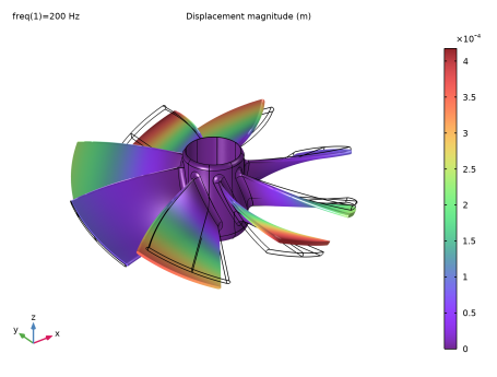
In the tree, select Frequency Domain Study (Full)/Solution 3 (sol3) > Solid Mechanics (Full) > Displacement (solid).
4
Click the Add Result Template button in the window toolbar.
Results
Displacement (solid)
In the Model Builder window, expand the Displacement (solid) node.
Deformation
1
In the Model Builder window, expand the Results > Displacement (solid) > Volume 1 node, then click Deformation.
2
In the Settings window for Deformation, locate the Scale section.
3
Select the Scale factor checkbox. In the associated text field, type 25.
4
In the Displacement (solid) toolbar, click  Plot.
Add Study
1
In the Home toolbar, click  Add Study to open the Add Study window.
2
Go to the Add Study window.
3
Find the Studies subsection. In the Select Study tree, select General Studies > Frequency Domain.
4
Find the Physics interfaces in study subsection. In the table, clear the Solve checkbox for Solid Mechanics (Full) (solid).
5
Click the Add Study button in the window toolbar.
6
In the Home toolbar, click  Add Study to close the Add Study window.
Study 4
Step 1: Frequency Domain
1
In the Settings window for Frequency Domain, locate the Study Settings section.
2
In the Frequencies text field, type 200.
3
Locate the Store in Output section. In the table, enter the following settings:
4
In the Model Builder window, click Study 4.
5
In the Settings window for Study, locate the Study Settings section.
6
Clear the Generate default plots checkbox.
7
In the Label text field, type Frequency Domain Study (Sector).
8
In the Study toolbar, click  Compute.
For a frequency-response analysis, use of the reduced geometry gives significant gains in both the memory required and computational time needed.
Results
Set up a displacement plot for the reduced geometry and compare it to that for the full geometry.
Result Templates
1
In the Home toolbar, click  Windows and choose Result Templates.
2
Go to the Result Templates window.
3
In the tree, select Frequency Domain Study (Sector)/Solution 4 (sol4) > Solid Mechanics (Sector) > Displacement, Full Geometry (solid2).
4
Click the Add Result Template button in the window toolbar.
Results
Displacement, Full Geometry (solid2)
In the Model Builder window, expand the Displacement, Full Geometry (solid2) node.
Deformation
1
In the Model Builder window, expand the Results > Displacement, Full Geometry (solid2) > Volume 1 node, then click Deformation.
2
In the Settings window for Deformation, locate the Scale section.
3
Select the Scale factor checkbox. In the associated text field, type 25.
4
In the Displacement, Full Geometry (solid2) toolbar, click  Plot.