
|
|
|

|
2E-9 m2/s
|
|
|
2E-6 m3/mol
|
|
|
1
|
|
2
|
|
3
|
Click Add.
|
|
4
|
|
5
|
Click Add.
|
|
6
|
Click
|
|
7
|
|
8
|
Click
|
|
1
|
|
2
|
|
4
|
|
1
|
|
2
|
|
3
|
Click
|
|
4
|
Browse to the model’s Application Libraries folder and double-click the file hydrogen_diffusion_parameters.txt.
|
|
5
|
|
1
|
|
2
|
|
3
|
|
1
|
|
2
|
|
3
|
|
4
|
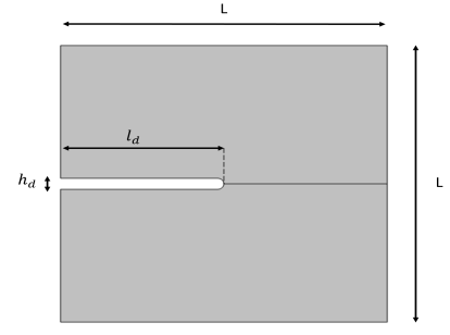
Click to expand the Layers section. In the table, enter the following settings:
|
|
5
|
|
1
|
|
2
|
|
3
|
|
4
|
|
5
|
|
6
|
|
1
|
|
2
|
On the object r1, select Points 2 and 3 only.
|
|
3
|
|
4
|
|
5
|
|
1
|
|
2
|
Select the object sq1 only.
|
|
3
|
|
4
|
|
5
|
Select the object fil1 only.
|
|
6
|
|
7
|
Click
|
|
1
|
|
2
|
Go to the Add Material window.
|
|
3
|
|
4
|
Click the Add to Component button in the window toolbar.
|
|
5
|
|
1
|
|
2
|
|
4
|
|
5
|
|
6
|
|
7
|
|
1
|
|
1
|
|
2
|
|
3
|
In the Expression text field, type (NT/N)*exp(Eb/(R_const*T0))/((1+(max(cl,0)/N)*exp(Eb/(R_const*T0)))^2).
|
|
4
|
|
5
|
|
7
|
|
8
|
|
1
|
|
2
|
|
3
|
Click
|
|
4
|
Browse to the model’s Application Libraries folder and double-click the file hydrogen_diffusion_variables.txt.
|
|
1
|
|
2
|
|
3
|
|
5
|
|
1
|
|
2
|
|
3
|
|
1
|
|
2
|
Click in the Graphics window and then press Ctrl+A to select both domains.
|
|
3
|
|
4
|
|
5
|
|
1
|
|
2
|
|
3
|
|
4
|
|
1
|
|
2
|
Click in the Graphics window and then press Ctrl+A to select both domains.
|
|
3
|
In the Settings window for Shrinkage and Swelling, locate the Shrinkage and Swelling Properties section.
|
|
4
|
|
1
|
|
2
|
|
3
|
|
1
|
|
3
|
|
4
|
|
5
|
|
6
|
|
1
|
|
3
|
|
4
|
|
5
|
|
6
|
|
7
|
|
1
|
|
2
|
|
3
|
|
1
|
|
3
|
|
4
|
Click to select the
|
|
6
|
Click
|
|
1
|
|
2
|
|
3
|
|
4
|
|
5
|
|
6
|
|
7
|
|
1
|
|
2
|
Go to the Add Study window.
|
|
3
|
|
4
|
Click the Add Study button in the window toolbar.
|
|
1
|
|
2
|
|
1
|
|
2
|
|
3
|
|
4
|
|
5
|
Locate the Physics and Variables Selection section. In the Solve for column of the table, under Component 1 (comp1) > Multiphysics, clear the checkbox for Shrinkage and Swelling 1 (sas1).
|
|
6
|
|
1
|
|
2
|
|
3
|
|
4
|
|
5
|
|
6
|
|
1
|
|
2
|
|
3
|
|
4
|
|
1
|
|
2
|
|
3
|
|
1
|
|
2
|
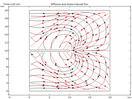
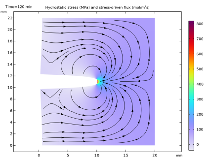
In the Settings window for Streamline, click Replace Expression in the upper-right corner of the Expression section. From the menu, choose Component 1 (comp1) > Transport in Solids > Species c > Fluxes > sas1.sflux_cx,sas1.sflux_cy - Stress-driven flux (spatial frame).
|
|
3
|
|
4
|
|
5
|
Locate the Coloring and Style section. Find the Point style subsection. From the Type list, choose Arrow.
|
|
6
|
|
1
|
|
2
|
|
1
|
|
2
|
|
3
|
|
4
|
|
5
|
|
6
|
|
1
|
|
2
|
|
3
|
|
1
|
|
2
|
|
3
|
|
4
|
|
5
|
Locate the Coloring and Style section. Find the Point style subsection. From the Color list, choose Black.
|
|
6
|
|
7
|
|
8
|
|
1
|
|
2
|
|
3
|
|
4
|
|
5
|
|
6
|
|
1
|
|
2
|
|
3
|
|
4
|
|
5
|
|
6
|
Locate the Coloring and Style section. Find the Point style subsection. From the Type list, choose Arrow.
|
|
1
|
|
2
|
|
3
|
|
4
|
|
5
|
Locate the Coloring and Style section. Find the Point style subsection. From the Color list, choose Red.
|
|
6
|
|
7
|
|
1
|
|
2
|
|
3
|
|
4
|
|
5
|
Locate the Plot Settings section.
|
|
6
|
|
7
|
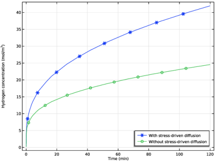
Select the y-axis label checkbox. In the associated text field, type Hydrogen concentration (mol/m<sup>3</sup>).
|
|
8
|
|
1
|
|
3
|
|
4
|
|
5
|
|
6
|
|
8
|
Click to expand the Coloring and Style section. Find the Line markers subsection. From the Marker list, choose Cycle.
|
|
9
|
|
1
|
|
2
|
|
3
|
|
4
|
|
5
|
Locate the Legends section. In the table, enter the following settings:
|
|
6
|
|
1
|
|
2
|
|
3
|
|
4
|
Locate the Plot Settings section.
|
|
5
|
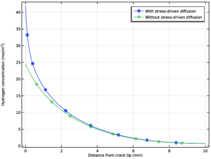
Select the y-axis label checkbox. In the associated text field, type Hydrogen concentration (mol/m<sup>3</sup>).
|
|
6
|
|
7
|
|
1
|
|
3
|
|
4
|
|
5
|
Click to expand the Coloring and Style section. Find the Line markers subsection. From the Marker list, choose Cycle.
|
|
6
|
|
7
|
|
8
|
|
1
|
|
2
|
|
3
|
|
4
|
Locate the Legends section. In the table, enter the following settings:
|
|
5
|
 ,
,