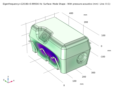
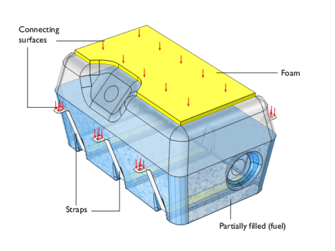
PDF

Fuel Tank Vibration
Introduction
This model analyzes the frequency response of a fuel tank partially filled with fluid. The tank is submitted to a vertical acceleration. Two modeling methods are considered to represent the fluid: a traditional method of smearing the mass of the fluid through the wetted surface of the fuel tank, and a multiphysics approach where the acoustic pressure within the fluid is specifically modeled.
The two methods show significant differences, highlighting how important it is to accurately capture the vibroacoustic behavior when predicting stress or fatigue life on fluid-filled cavities.
Model Definition
Fluids can have a substantial influence on the vibrational behavior of structures. This tutorial compares two modeling approaches:
Figure 1: Geometry of the fuel tank showing the different domains and the boundaries subject to the displacement source.
Traditionally, fluid masses have been considered as nonstructural masses added to the wetted surfaces, with the assumption that this was a conservative approach. A more precise approach involves modeling the fluid using pressure acoustics. That is, solving for the pressure waves in the fluid. The multiphysics coupling between fluid and structure is automatically handled in COMSOL Multiphysics. This results in a model where the mass of the fluid as well as its compliance is fully included in the model. Combined acoustic and structural modes are hence also captured in full detail.
The fuel tank is secured to the surrounding structure through a foam block and three fuel tank straps bolted at their end. The fuel tank is partially filled, as seen in Figure 1.
A unit vertical displacement is applied to the boundaries in contact with the surrounds (red arrows in Figure 1). This excitation is swept through a frequency range to obtain the frequency response function (FRF) of any variable. The FRF can be used to obtain the response of the fuel tank against any frequency dependent load.
Figure 2: The frequency response function (FRF) evaluated at the mounting strap.
Results and Discussion
The frequency response function (FRF), here representing the transfer function from the applied displacement to the zz-component of the stress at the mounting strap, is depicted in Figure 2. The plot shows the results of the two modeling approaches, and it is clear to see that they diverge greatly.
The absolute stress of the fuel tank computed at two significant resonance frequencies seen in the FRF (one from each method) is depicted in Figure 3 and Figure 4, respectively. The first figure shows the response at 90 Hz, while the second shows the response at 127.5 Hz. Both peaks are clearly seen in the FRF plot.
The location of the resonance peaks are also captured in the eigenfrequency analysis carried out in the model in Study 1 and Study 2.
Figure 3: Stress evaluated at 90 Hz, corresponding to the first peak in the FRF of the full multiphysics model.
Figure 4: Stress evaluated at 127.5 Hz, corresponding to the first major peak in the FRF of the model solved with added mass.
Application Library path: Structural_Mechanics_Module/Fluid-Structure_Interaction/fuel_tank_vibration
Modeling Instructions
From the File menu, choose New.
New
In the New window, click  Model Wizard.
Model Wizard
1
In the Model Wizard window, click  3D.
2
In the Select Physics tree, select Structural Mechanics > Shell (shell).
3
Click Add.
4
In the Select Physics tree, select Structural Mechanics > Solid Mechanics (solid).
5
Click Add.
6
In the Select Physics tree, select Acoustics > Pressure Acoustics > Pressure Acoustics, Frequency Domain (acpr).
7
Click Add.
8
Click  Study.
9
In the Select Study tree, select General Studies > Eigenfrequency.
10
Global Definitions
Parameters 1
1
In the Model Builder window, under Global Definitions click Parameters 1.
2
In the Settings window for Parameters, locate the Parameters section.
3
Click  Load from File.
4
Geometry 1
The geometry sequence for the model is available in a file. Insert it as follows:
1
In the Model Builder window, under Component 1 (comp1) click Geometry 1.
2
In the Settings window for Geometry, locate the Units section.
3
From the Length unit list, choose mm.
Import 1 (imp1)
1
In the Geometry toolbar, click  Import.
2
In the Settings window for Import, locate the Source section.
3
Click  Browse.
4
5
Click  Import.
6
In the Geometry toolbar, click  Build All.
Disable the analysis of the geometry as the remaining small geometric details can be kept.
7
In the Model Builder window, click Geometry 1.
8
In the Settings window for Geometry, locate the Cleanup section.
9
Clear the Automatic detection of small details checkbox.
10
In the Geometry toolbar, click  Build All.
Definitions
Straps
1
In the Model Builder window, expand the Component 1 (comp1) > Definitions node.
2
Right-click Definitions and choose Selections > Explicit.
3
In the Settings window for Explicit, type Straps in the Label text field.
4
Click the  Wireframe Rendering button in the Graphics toolbar.
5
Locate the Input Entities section. From the Geometric entity level list, choose Boundary.
6
7
Select the Group by continuous tangent checkbox.
Fuel Tank
1
In the Definitions toolbar, click  Explicit.
2
In the Settings window for Explicit, type Fuel Tank in the Label text field.
3
Locate the Input Entities section. From the Geometric entity level list, choose Boundary.
4
Click  Paste Selection.
5
In the Paste Selection dialog, type 10-12, 14-82, 86-91, 104-113, 116, 122-126, 129, 131-150, 152-156, 158-162, 164-168, 170-172, 179-202 in the Selection text field.
6
Foam
1
In the Definitions toolbar, click  Explicit.
2
In the Settings window for Explicit, type Foam in the Label text field.
3
Locate the Input Entities section. Click  Paste Selection.
4
In the Paste Selection dialog, type 3-6 in the Selection text field.
5
Shells
1
In the Definitions toolbar, click  Union.
2
In the Settings window for Union, type Shells in the Label text field.
3
Locate the Geometric Entity Level section. From the Level list, choose Boundary.
4
Locate the Input Entities section. Under Selections to add, click  Add.
5
In the Add dialog, select Straps in the Selections to add list.
6
7
In the Settings window for Union, locate the Input Entities section.
8
Under Selections to add, click  Add.
9
In the Add dialog, select Fuel Tank in the Selections to add list.
10
Fuel
1
In the Definitions toolbar, click  Explicit.
2
In the Settings window for Explicit, type Fuel in the Label text field.
3
Wetted Surface
1
In the Definitions toolbar, click  Explicit.
2
In the Settings window for Explicit, type Wetted Surface in the Label text field.
3
Locate the Input Entities section. From the Geometric entity level list, choose Boundary.
4
Click  Paste Selection.
5
In the Paste Selection dialog, type 12, 14, 16, 22-36, 46-79, 90, 91, 104-112, 125, 126, 131-148, 155, 156, 158-162, 164-168, 170-172, 179-201 in the Selection text field.
6
Attached Boundaries
1
In the Definitions toolbar, click  Explicit.
2
In the Settings window for Explicit, type Attached Boundaries in the Label text field.
3
Locate the Input Entities section. From the Geometric entity level list, choose Boundary.
4
Click  Paste Selection.
5
In the Paste Selection dialog, type 1-3, 117, 206-208 in the Selection text field.
6
Fluid Free Surface
1
In the Definitions toolbar, click  Explicit.
2
In the Settings window for Explicit, type Fluid Free Surface in the Label text field.
3
Locate the Input Entities section. From the Geometric entity level list, choose Boundary.
4
Click  Paste Selection.
5
In the Paste Selection dialog, type 13 in the Selection text field.
6
Fuel Mass
1
Right-click Definitions and choose Physics Utilities > Mass Properties.
2
In the Settings window for Mass Properties, type Fuel Mass in the Label text field.
3
Locate the Source Selection section. From the Selection list, choose Fuel.
4
Locate the Density section. In the Density expression text field, type rho0.
Add Material
1
In the Home toolbar, click  Add Material to open the Add Material window.
2
Go to the Add Material window.
3
In the tree, select Built-in > Aluminum 6063-T83.
4
Click the Add to Component button in the window toolbar.
5
In the tree, select Built-in > Steel AISI 4340.
6
Click the Add to Component button in the window toolbar.
7
In the Home toolbar, click  Add Material to close the Add Material window.
Materials
Aluminum 6063-T83 (mat1)
1
In the Settings window for Material, locate the Geometric Entity Selection section.
2
From the Geometric entity level list, choose Boundary.
3
From the Selection list, choose Fuel Tank.
4
Click to expand the Material Properties section. In the Material properties tree, select Basic Properties > Isotropic Structural Loss Factor.
5
Click  Add to Material.
6
Locate the Material Contents section. In the table, enter the following settings:
Steel AISI 4340 (mat2)
1
In the Model Builder window, click Steel AISI 4340 (mat2).
2
In the Settings window for Material, locate the Geometric Entity Selection section.
3
From the Geometric entity level list, choose Boundary.
4
From the Selection list, choose Straps.
5
Click to expand the Material Properties section. In the Material properties tree, select Basic Properties > Isotropic Structural Loss Factor.
6
Click  Add to Material.
7
Locate the Material Contents section. In the table, enter the following settings:
Fuel
1
In the Materials toolbar, click  Blank Material.
2
In the Settings window for Material, type Fuel in the Label text field.
3
Locate the Geometric Entity Selection section. From the Selection list, choose Fuel.
4
Locate the Material Contents section. In the table, enter the following settings:
Foam Material
1
In the Materials toolbar, click  Blank Material.
2
In the Settings window for Material, type Foam Material in the Label text field.
3
Locate the Geometric Entity Selection section. From the Selection list, choose Foam.
4
Locate the Material Contents section. In the table, enter the following settings:
5
Click to expand the Material Properties section. In the Material properties tree, select Basic Properties > Isotropic Structural Loss Factor.
6
Click  Add to Material.
7
Locate the Material Contents section. In the table, enter the following settings:
Shell (shell)
1
In the Model Builder window, under Component 1 (comp1) click Shell (shell).
2
In the Settings window for Shell, locate the Boundary Selection section.
3
From the Selection list, choose Shells.
Linear Elastic Material 1
1
In the Model Builder window, expand the Shell (shell) node.
2
In the Model Builder window, click Linear Elastic Material 1.
Damping 1
1
In the Physics toolbar, click  Attributes and choose Damping.
2
In the Settings window for Damping, locate the Damping Settings section.
3
From the Damping type list, choose Isotropic loss factor.
Thickness and Offset 1
1
In the Model Builder window, under Component 1 (comp1) > Shell (shell) click Thickness and Offset 1.
2
In the Settings window for Thickness and Offset, locate the Thickness and Offset section.
3
In the d0 text field, type wall_th.
Thickness and Offset 2
1
In the Physics toolbar, click  Boundaries and choose Thickness and Offset.
2
In the Settings window for Thickness and Offset, locate the Boundary Selection section.
3
From the Selection list, choose Straps.
4
Locate the Thickness and Offset section. In the d0 text field, type strap_th.
Added Mass 1
1
In the Physics toolbar, click  Boundaries and choose Added Mass.
2
In the Settings window for Added Mass, locate the Boundary Selection section.
3
From the Selection list, choose Wetted Surface.
4
Locate the Added Mass section. From the Mass type list, choose Total mass.
5
In the m text field, type mass1.mass.
Prescribed Displacement/Rotation 1
1
In the Physics toolbar, click  Boundaries and choose Prescribed Displacement/Rotation.
2
In the Settings window for Prescribed Displacement/Rotation, locate the Boundary Selection section.
3
From the Selection list, choose Attached Boundaries.
4
Locate the Prescribed Displacement section. From the Displacement in x direction list, choose Prescribed.
5
From the Displacement in y direction list, choose Prescribed.
6
From the Displacement in z direction list, choose Prescribed.
7
In the u0z text field, type d0.
The prescribed displacement represents a harmonic source of (complex valued) amplitude d0 in a frequency domain study. In an eigenfrequency study, the prescribed displacement is interpreted as a constraint with zero amplitude, that is, a fixed constraint. Loads are zero in eigenfrequency studies.
Solid Mechanics (solid)
1
In the Model Builder window, under Component 1 (comp1) click Solid Mechanics (solid).
2
In the Settings window for Solid Mechanics, locate the Domain Selection section.
3
From the Selection list, choose Foam.
Linear Elastic Material 1
In the Model Builder window, expand the Solid Mechanics (solid) node, then click Linear Elastic Material 1.
Damping 1
1
In the Physics toolbar, click  Attributes and choose Damping.
2
In the Settings window for Damping, locate the Damping Settings section.
3
From the Damping type list, choose Isotropic loss factor.
Prescribed Displacement 1
1
In the Physics toolbar, click  Boundaries and choose Prescribed Displacement.
2
In the Settings window for Prescribed Displacement, locate the Boundary Selection section.
3
From the Selection list, choose Attached Boundaries.
4
Locate the Prescribed Displacement section. From the Displacement in x direction list, choose Prescribed.
5
From the Displacement in y direction list, choose Prescribed.
6
From the Displacement in z direction list, choose Prescribed.
7
In the u0z text field, type d0.
Pressure Acoustics, Frequency Domain (acpr)
1
In the Model Builder window, under Component 1 (comp1) click Pressure Acoustics, Frequency Domain (acpr).
2
In the Settings window for Pressure Acoustics, Frequency Domain, locate the Domain Selection section.
3
From the Selection list, choose Fuel.
Sound Soft Boundary 1
1
In the Physics toolbar, click  Boundaries and choose Sound Soft Boundary.
2
In the Settings window for Sound Soft Boundary, locate the Boundary Selection section.
3
From the Selection list, choose Fluid Free Surface.
Proceed to set up the Multiphysics Couplings that couple the Solid Mechanics and the Pressure Acoustics, Frequency Domain to the Shell thin structure.
Multiphysics
Solid–Thin Structure Connection 1 (sshc1)
1
In the Physics toolbar, click  Multiphysics Couplings and choose Global > Solid–Thin Structure Connection.
2
In the Settings window for Solid–Thin Structure Connection, locate the Connection Settings section.
3
From the Connection type list, choose Shared boundaries.
Acoustic–Structure Boundary 1 (asb1)
1
In the Physics toolbar, click  Multiphysics Couplings and choose Boundary > Acoustic–Structure Boundary.
2
In the Settings window for Acoustic–Structure Boundary, locate the Boundary Selection section.
3
From the Selection list, choose Wetted Surface.
Mesh 1
In this model, the mesh is set up manually. Proceed by directly adding the desired mesh components.
Mapped 1
1
In the Mesh toolbar, click  More Generators and choose Mapped.
2
In the Settings window for Mapped, locate the Boundary Selection section.
3
Click  Paste Selection.
4
In the Paste Selection dialog, type 7-9, 11, 14-21, 40, 43, 46-53, 55, 58, 61, 63, 71-78, 83-89, 91, 101, 104-110, 112, 113, 122-126, 129, 131-136, 139-148, 150, 152, 154, 173-179, 181, 183, 184, 186, 188, 189, 191, 193, 194, 202 in the Selection text field.
5
Size 1
1
Right-click Mapped 1 and choose Size.
2
In the Settings window for Size, locate the Element Size section.
3
Click the Custom button.
4
Locate the Element Size Parameters section.
5
Select the Maximum element size checkbox. In the associated text field, type mesh_size.
6
Select the Minimum element size checkbox. In the associated text field, type mesh_size/min_mesh_factor.
Free Quad 1
1
In the Mesh toolbar, click  More Generators and choose Free Quad.
2
Size 1
1
Right-click Free Quad 1 and choose Size.
2
In the Settings window for Size, locate the Element Size section.
3
Click the Custom button.
4
Locate the Element Size Parameters section.
5
Select the Maximum element size checkbox. In the associated text field, type mesh_size.
6
Select the Minimum element size checkbox. In the associated text field, type mesh_size/min_mesh_factor.
Size
1
In the Model Builder window, under Component 1 (comp1) > Mesh 1 click Size.
2
In the Settings window for Size, locate the Element Size section.
3
Click the Custom button.
In general, 5 to 6 second-order elements per wavelength are needed to resolve the waves. For more details, see Meshing (Resolving the Waves) in the Acoustics Module User’s Guide . In this model, use 5 elements per wavelength. Use the wavelength at maximum frequency.
4
Locate the Element Size Parameters section. In the Maximum element size text field, type lam0/6.
5
In the Minimum element size text field, type 6[mm].
Swept 1
1
In the Mesh toolbar, click  Swept.
2
In the Settings window for Swept, locate the Domain Selection section.
3
From the Geometric entity level list, choose Domain.
4
From the Selection list, choose Foam.
Free Tetrahedral 1
1
In the Mesh toolbar, click  Free Tetrahedral.
2
In the Settings window for Free Tetrahedral, locate the Domain Selection section.
3
From the Geometric entity level list, choose Domain.
4
From the Selection list, choose Fuel.
5
Click to expand the Element Quality Optimization section. Clear the Avoid inverted curved elements checkbox.
Size 1
1
Right-click Free Tetrahedral 1 and choose Size.
2
In the Settings window for Size, locate the Geometric Entity Selection section.
3
From the Geometric entity level list, choose Boundary.
4
From the Selection list, choose Wetted Surface.
5
Locate the Element Size section. Click the Custom button.
6
Locate the Element Size Parameters section.
7
Select the Maximum element size checkbox. In the associated text field, type mesh_size.
8
Select the Minimum element size checkbox. In the associated text field, type mesh_size/min_mesh_factor.
Free Triangular 1
1
In the Mesh toolbar, click  More Generators and choose Free Triangular.
2
In the Settings window for Free Triangular, locate the Boundary Selection section.
3
From the Geometric entity level list, choose Remaining.
4
Click  Build All.
Traditionally, fluid masses have been considered as nonstructural masses added to the wetted surfaces, with the assumption that this was a conservative approach. A more precise approach involves modeling the fluid through the Pressure Acoustics physics. Study 1 and 3 correspond to the modes and the frequency response in the case of the added mass, while study 2 and 4 are the modes and frequency response with the acoustic domain.
Study 1 - Modes with Added Mass
1
In the Model Builder window, click Study 1.
2
In the Settings window for Study, type Study 1 - Modes with Added Mass in the Label text field.
3
Locate the Study Settings section. Clear the Generate default plots checkbox.
Turn off the generation of default plots. If turned on, the default plots for each physics interface will be generated.
Step 1: Eigenfrequency
1
In the Model Builder window, expand the Study 1 - Modes with Added Mass node, then click Step 1: Eigenfrequency.
2
In the Settings window for Eigenfrequency, locate the Study Settings section.
3
Select the Desired number of eigenfrequencies checkbox.
4
In the Search for eigenfrequencies around shift text field, type 0[Hz].
5
Locate the Physics and Variables Selection section. In the Solve for column of the table, under Component 1 (comp1), clear the checkbox for Pressure Acoustics, Frequency Domain (acpr).
6
In the Solve for column of the table, under Component 1 (comp1) > Multiphysics, clear the checkbox for Acoustic–Structure Boundary 1 (asb1).
Add Study
1
In the Study toolbar, click  Add Study to open the Add Study window.
2
Go to the Add Study window.
3
Find the Studies subsection. In the Select Study tree, select General Studies > Eigenfrequency.
4
Click the Add Study button in the window toolbar.
5
In the Select Study tree, select General Studies > Frequency Domain.
6
Click the Add Study button in the window toolbar.
7
Click the Add Study button in the window toolbar.
8
In the Study toolbar, click  Add Study to close the Add Study window.
Study 2 - Modes with Acoustic
1
In the Settings window for Study, type Study 2 - Modes with Acoustic in the Label text field.
2
Locate the Study Settings section. Clear the Generate default plots checkbox.
1
In the Model Builder window, under Study 2 - Modes with Acoustic click Step 1: Eigenfrequency.
2
In the Settings window for Eigenfrequency, locate the Study Settings section.
3
Select the Desired number of eigenfrequencies checkbox.
4
In the Search for eigenfrequencies around shift text field, type 0[Hz].
5
Locate the Physics and Variables Selection section. Select the Modify model configuration for study step checkbox.
6
In the tree, select Component 1 (comp1) > Shell (shell) > Added Mass 1.
7
Study 3 - Frequency Response with Added Mass
1
In the Model Builder window, click Study 3.
2
In the Settings window for Study, type Study 3 - Frequency Response with Added Mass in the Label text field.
3
Locate the Study Settings section. Clear the Generate default plots checkbox.
Step 1: Frequency Domain
1
In the Model Builder window, under Study 3 - Frequency Response with Added Mass click Step 1: Frequency Domain.
2
In the Settings window for Frequency Domain, locate the Study Settings section.
3
Click  Range.
4
In the Range dialog, type fmin in the Start text field.
5
In the Step text field, type deltaf.
6
In the Stop text field, type fmax.
7
Click Add.
8
In the Settings window for Frequency Domain, locate the Physics and Variables Selection section.
9
In the Solve for column of the table, under Component 1 (comp1), clear the checkbox for Pressure Acoustics, Frequency Domain (acpr).
10
In the Solve for column of the table, under Component 1 (comp1) > Multiphysics, clear the checkbox for Acoustic–Structure Boundary 1 (asb1).
Study 4 - Frequency Response with Acoustics
1
In the Model Builder window, click Study 4.
2
In the Settings window for Study, locate the Study Settings section.
3
Clear the Generate default plots checkbox.
4
In the Label text field, type Study 4 - Frequency Response with Acoustics.
1
In the Model Builder window, under Study 4 - Frequency Response with Acoustics click Step 1: Frequency Domain.
2
In the Settings window for Frequency Domain, locate the Study Settings section.
3
Click  Range.
4
In the Range dialog, type fmin in the Start text field.
5
In the Step text field, type deltaf.
6
In the Stop text field, type fmax.
7
Click Add.
8
In the Settings window for Frequency Domain, locate the Physics and Variables Selection section.
9
Select the Modify model configuration for study step checkbox.
10
In the tree, select Component 1 (comp1) > Shell (shell) > Added Mass 1.
11
Now, compute the four studies.
Study 1 - Modes with Added Mass
In the Study toolbar, click  Compute.
Study 2 - Modes with Acoustic
Click  Compute.
Study 3 - Frequency Response with Added Mass
Click  Compute.
Study 4 - Frequency Response with Acoustics
Click  Compute.
Results
Mode Shape with Added Mass
1
In the Results toolbar, click  3D Plot Group.
2
In the Settings window for 3D Plot Group, type Mode Shape with Added Mass in the Label text field.
3
Locate the Data section. From the Eigenfrequency (Hz) list, choose 113.98+0.77305i.
4
Locate the Plot Settings section. Clear the Plot dataset edges checkbox.
5
Locate the Color Legend section. Clear the Show legends checkbox.
Surface 1
1
In the Mode Shape with Added Mass toolbar, click  Surface.
2
In the Settings window for Surface, locate the Expression section.
3
In the Expression text field, type if(isnan(solid.disp),shell.disp,solid.disp).
4
Select the Description checkbox. In the associated text field, type Mode Shape - With added mass.
5
Locate the Coloring and Style section. From the Color table list, choose AuroraBorealis.
Deformation 1
1
In the Mode Shape with Added Mass toolbar, click  Deformation.
2
In the Settings window for Deformation, locate the Expression section.
3
In the X-component text field, type if(isnan(u2),u,u2).
4
In the Y-component text field, type if(isnan(v2),v,v2).
5
In the Z-component text field, type if(isnan(w2),w,w2).
Mode Shape with Added Mass
In the Mode Shape with Added Mass toolbar, click  Line.
Line 1
1
In the Settings window for Line, locate the Expression section.
2
In the Expression text field, type 0.
3
Locate the Coloring and Style section. From the Coloring list, choose Uniform.
4
From the Color list, choose Black.
5
Click to expand the Inherit Style section. From the Plot list, choose Surface 1.
6
Clear the Color checkbox.
7
Clear the Color and data range checkbox.
Deformation 1
1
In the Mode Shape with Added Mass toolbar, click  Deformation.
2
In the Settings window for Deformation, locate the Expression section.
3
In the X-component text field, type if(isnan(u2),u,u2).
4
In the Y-component text field, type if(isnan(v2),v,v2).
5
In the Z-component text field, type if(isnan(w2),w,w2).
Mode Shape with Added Mass
1
In the Model Builder window, under Results click Mode Shape with Added Mass.
2
In the Mode Shape with Added Mass toolbar, click  Plot.
Mode Shape with Acoustics
1
Right-click Mode Shape with Added Mass and choose Duplicate.
2
In the Settings window for 3D Plot Group, type Mode Shape with Acoustics in the Label text field.
3
Locate the Data section. From the Dataset list, choose Study 2 - Modes with Acoustic/Solution 2 (sol2).
4
From the Eigenfrequency (Hz) list, choose 120.72+1.0002i.
Surface 1
1
In the Model Builder window, expand the Mode Shape with Acoustics node, then click Surface 1.
2
In the Settings window for Surface, locate the Expression section.
3
In the Description text field, type Mode Shape - With pressure acoustics.
Mode Shape with Acoustics
1
In the Model Builder window, click Mode Shape with Acoustics.
2
In the Mode Shape with Acoustics toolbar, click  Plot.
FRF: Stress at the Fuel Tank Strap
1
In the Home toolbar, click  Add Plot Group and choose 1D Plot Group.
2
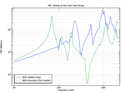
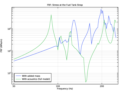
In the Settings window for 1D Plot Group, type FRF: Stress at the Fuel Tank Strap in the Label text field.
3
Click to expand the Title section. From the Title type list, choose Label.
4
Locate the Data section. From the Dataset list, choose Study 3 - Frequency Response with Added Mass/Solution 3 (sol3).
5
Locate the Plot Settings section.
6
Select the x-axis label checkbox. In the associated text field, type Frequency (Hz).
7
Select the y-axis label checkbox. In the associated text field, type FRF (MPa/m).
8
Locate the Axis section. Select the x-axis log scale checkbox.
9
Select the y-axis log scale checkbox.
10
Locate the Legend section. From the Position list, choose Lower left.
Octave Band 1
1
In the FRF: Stress at the Fuel Tank Strap toolbar, click  More Plots and choose Octave Band.
2
3
In the Settings window for Octave Band, locate the y-Axis Data section.
4
In the Expression text field, type abs(shell.szz)/1e9.
5
From the Expression type list, choose General (non-dB).
6
In the Reference expression text field, type d0.
7
Locate the Plot section. From the Quantity list, choose Continuous power spectral density.
8
Click to expand the Legends section. Select the Show legends checkbox.
9
From the Legends list, choose Manual.
10
Octave Band 2
1
Right-click Octave Band 1 and choose Duplicate.
2
In the Settings window for Octave Band, locate the Data section.
3
From the Dataset list, choose Study 4 - Frequency Response with Acoustics/Solution 4 (sol4).
4
Locate the Legends section. In the table, enter the following settings:
5
In the FRF: Stress at the Fuel Tank Strap toolbar, click  Plot.
The stress for one point of the fuel tank straps should look like the following figure:
Absolute Stress Comparison at 90 Hz
1
In the Home toolbar, click  Add Plot Group and choose 3D Plot Group.
2
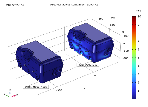
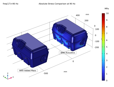
In the Settings window for 3D Plot Group, type Absolute Stress Comparison at 90 Hz in the Label text field.
3
Locate the Data section. From the Dataset list, choose Study 4 - Frequency Response with Acoustics/Solution 4 (sol4).
4
From the Parameter value (freq (Hz)) list, choose 90.
5
Click to expand the Title section. From the Title type list, choose Label.
6
Locate the Color Legend section. Select the Show units checkbox.
7
Locate the Plot Settings section. Clear the Plot dataset edges checkbox.
Surface 1
1
In the Absolute Stress Comparison at 90 Hz toolbar, click  Surface.
2
In the Settings window for Surface, locate the Expression section.
3
In the Expression text field, type if(isnan(solid.SZZ),abs(shell.szz),abs(solid.SZZ)).
4
From the Unit list, choose MPa.
5
Click to expand the Range section. Select the Manual color range checkbox.
6
In the Maximum text field, type 10.
7
Locate the Coloring and Style section. From the Color table list, choose Rainbow.
Deformation 1
1
In the Absolute Stress Comparison at 90 Hz toolbar, click  Deformation.
2
In the Settings window for Deformation, locate the Expression section.
3
In the X-component text field, type if(isnan(u2),u,u2).
4
In the Y-component text field, type if(isnan(v2),v,v2).
5
In the Z-component text field, type if(isnan(w2),w,w2).
6
Locate the Scale section.
7
Select the Scale factor checkbox. In the associated text field, type 250.
Absolute Stress Comparison at 90 Hz
In the Absolute Stress Comparison at 90 Hz toolbar, click  Line.
Line 1
1
In the Settings window for Line, locate the Expression section.
2
In the Expression text field, type 0.
3
Locate the Coloring and Style section. From the Coloring list, choose Uniform.
4
From the Color list, choose Black.
5
Locate the Inherit Style section. From the Plot list, choose Surface 1.
6
Clear the Color checkbox.
7
Clear the Color and data range checkbox.
Deformation 1
1
In the Absolute Stress Comparison at 90 Hz toolbar, click  Deformation.
2
In the Settings window for Deformation, locate the Expression section.
3
In the X-component text field, type if(isnan(u2),u,u2).
4
In the Y-component text field, type if(isnan(v2),v,v2).
5
In the Z-component text field, type if(isnan(w2),w,w2).
Absolute Stress Comparison at 90 Hz
In the Absolute Stress Comparison at 90 Hz toolbar, click  Annotation.
Annotation 1
1
In the Settings window for Annotation, locate the Annotation section.
2
In the Text text field, type With Acoustics.
3
Locate the Position section. In the Y text field, type 100.
4
In the Z text field, type -200.
5
Locate the Coloring and Style section. Clear the Show point checkbox.
6
From the Anchor point list, choose Center.
7
Select the Show frame checkbox.
Absolute Stress Comparison at 90 Hz
In the Absolute Stress Comparison at 90 Hz toolbar, click  Surface.
Surface 2
1
In the Settings window for Surface, locate the Data section.
2
From the Dataset list, choose Study 3 - Frequency Response with Added Mass/Solution 3 (sol3).
3
From the Parameter value (freq (Hz)) list, choose 90.
4
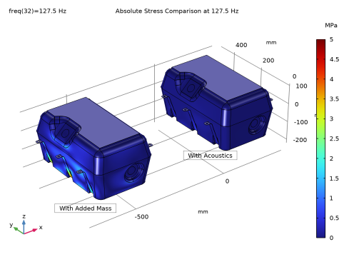
Locate the Expression section. In the Expression text field, type if(isnan(solid.SZZ),abs(shell.szz),abs(solid.SZZ)).
5
From the Unit list, choose MPa.
6
Click to expand the Inherit Style section. From the Plot list, choose Surface 1.
Deformation 1
1
In the Absolute Stress Comparison at 90 Hz toolbar, click  Deformation.
2
In the Settings window for Deformation, locate the Expression section.
3
In the X-component text field, type if(isnan(u2),u,u2).
4
In the Y-component text field, type if(isnan(v2),v,v2).
5
In the Z-component text field, type if(isnan(w2),w,w2).
Surface 2
In the Model Builder window, click Surface 2.
Transformation 1
1
In the Absolute Stress Comparison at 90 Hz toolbar, click  More Attributes and choose Transformation.
2
In the Settings window for Transformation, locate the Transformation section.
3
In the X text field, type -700.
Absolute Stress Comparison at 90 Hz
In the Absolute Stress Comparison at 90 Hz toolbar, click  Line.
Line 2
1
In the Settings window for Line, locate the Expression section.
2
In the Expression text field, type 0.
3
Locate the Data section. From the Dataset list, choose Study 3 - Frequency Response with Added Mass/Solution 3 (sol3).
4
From the Parameter value (freq (Hz)) list, choose 90.
5
Locate the Coloring and Style section. From the Coloring list, choose Uniform.
6
From the Color list, choose Black.
7
Locate the Inherit Style section. Clear the Color checkbox.
8
Clear the Color and data range checkbox.
9
From the Plot list, choose Surface 2.
Deformation 1
1
In the Absolute Stress Comparison at 90 Hz toolbar, click  Deformation.
2
In the Settings window for Deformation, locate the Expression section.
3
In the X-component text field, type if(isnan(u2),u,u2).
4
In the Y-component text field, type if(isnan(v2),v,v2).
5
In the Z-component text field, type if(isnan(w2),w,w2).
Line 2
In the Model Builder window, click Line 2.
Transformation 1
1
In the Absolute Stress Comparison at 90 Hz toolbar, click  More Attributes and choose Transformation.
2
In the Settings window for Transformation, locate the Transformation section.
3
In the X text field, type -700.
Absolute Stress Comparison at 90 Hz
In the Absolute Stress Comparison at 90 Hz toolbar, click  Annotation.
Annotation 2
1
In the Settings window for Annotation, locate the Annotation section.
2
In the Text text field, type With Added Mass.
3
Locate the Position section. In the X text field, type -700.
4
In the Y text field, type 100.
5
In the Z text field, type -220.
6
Locate the Coloring and Style section. Clear the Show point checkbox.
7
Select the Show frame checkbox.
8
From the Anchor point list, choose Center.
Absolute Stress Comparison at 90 Hz
1
In the Model Builder window, click Absolute Stress Comparison at 90 Hz.
2
In the Absolute Stress Comparison at 90 Hz toolbar, click  Plot.
The stress comparison between the added mass fluid and the acoustic domain at f=90 Hz should look like the following figure:
Absolute Stress Comparison at 127.5 Hz
1
Right-click Absolute Stress Comparison at 90 Hz and choose Duplicate.
2
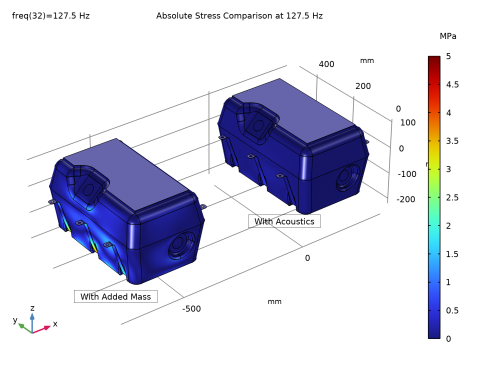
In the Settings window for 3D Plot Group, type Absolute Stress Comparison at 127.5 Hz in the Label text field.
3
Locate the Data section. From the Parameter value (freq (Hz)) list, choose 127.5.
Surface 1
1
In the Model Builder window, expand the Absolute Stress Comparison at 127.5 Hz node, then click Surface 1.
2
In the Settings window for Surface, locate the Range section.
3
In the Maximum text field, type 5.
Surface 2
1
In the Model Builder window, click Surface 2.
2
In the Settings window for Surface, locate the Data section.
3
From the Parameter value (freq (Hz)) list, choose 127.5.
Line 2
1
In the Model Builder window, click Line 2.
2
In the Settings window for Line, locate the Data section.
3
From the Parameter value (freq (Hz)) list, choose 127.5.
Absolute Stress Comparison at 127.5 Hz
1
In the Model Builder window, click Absolute Stress Comparison at 127.5 Hz.
2
In the Absolute Stress Comparison at 127.5 Hz toolbar, click  Plot.
The stress comparison between the added mass fluid and the acoustic domain at f=127.5 Hz should look like the following figure:
Eigenfrequencies with Added Mass
1
In the Results toolbar, click  Evaluation Group.
2
In the Settings window for Evaluation Group, type Eigenfrequencies with Added Mass in the Label text field.
Global Evaluation 1
1
In the Eigenfrequencies with Added Mass toolbar, click  Global Evaluation.
2
In the Settings window for Global Evaluation, locate the Expressions section.
3
4
In the Eigenfrequencies with Added Mass toolbar, click  Evaluate.
Eigenfrequencies with Acoustics
1
In the Model Builder window, right-click Eigenfrequencies with Added Mass and choose Duplicate.
2
In the Settings window for Evaluation Group, type Eigenfrequencies with Acoustics in the Label text field.
3
Locate the Data section. From the Dataset list, choose Study 2 - Modes with Acoustic/Solution 2 (sol2).
4
In the Eigenfrequencies with Acoustics toolbar, click  Evaluate.
Fuel Mass Evaluation
1
In the Results toolbar, click  Evaluation Group.
2
In the Settings window for Evaluation Group, type Fuel Mass Evaluation in the Label text field.
3
Locate the Data section. From the Eigenfrequency selection list, choose Last.
Global Evaluation 1
1
Right-click Fuel Mass Evaluation and choose Global Evaluation.
2
In the Settings window for Global Evaluation, locate the Expressions section.
3
4
In the Fuel Mass Evaluation toolbar, click  Evaluate.
The final two plots are optional and the instructions for generating them are skipped here. The first is the thumbnail image used for the model; and the second generates a geometry overview plot. Click on the plots in the model to see how they are generated.