PDF

Eigenfrequency Shifts Caused by Temperature Changes
Introduction
Some devices require a very high degree of frequency stability with respect to changes in the environment. In some applications, particularly within the MEMS field, it is important to study the sensitivity of a device’s eigenfrequencies with respect to a variation in temperature. The same type of phenomena could, for example, also be caused by hygroscopic swelling due to changes in humidity. In very high precision applications, the frequency stability requirements might specify a precision at the ppb (parts-per-billion, 10−9) level. Setting up simulations that accurately capture such small effects can be a challenging task, since several phenomena can interact.
This COMSOL Multiphysics example shows how to perform a sensitivity analysis of the eigenfrequencies of a beam subjected to thermal expansion. Effects like stress softening, geometric changes, and the temperature dependence of material properties are explored.
Model Definition
Consider a rectangular beam with the data listed in Table 1.
ν
ρ
αx
1·10-5 1/K
2·10-5 1/K
3·10-5 1/K
The material parameters have values that are of the same order of magnitude as those for many other engineering materials. To better separate the various effects, Poisson’s ratio is set to zero, but this assumption does not change the results in any fundamental way. Orthotropic thermal expansion coefficients are used to highlight some properties of the solution.
Results and Discussion
The eigenfrequencies of the beam are computed for two different types of boundary conditions: a doubly clamped beam, and a cantilever beam, where one end is fixed and the other end is free.
The mode shapes of the doubly clamped beam are shown in Figure 1.
Figure 1: Mode shapes for the doubly clamped beam.
The eigenfrequencies computed for the doubly clamped beam, without any thermal expansion, are listed in Table 2 along with the eigenfrequencies obtained with a temperature rise of 10 K, and the ratio between the two.
Figure 2 shows the shift in frequency as a function of the temperature variation.
Figure 2: Frequency shift as a function of the temperature change for the doubly clamped beam.
Stress softening effect
The first thing to note is that the bending eigenmodes for the doubly clamped beam stand out and have a strong temperature dependence. If a thinner beam is considered, this difference would be even more pronounced. The reason for this behavior is related to the fact that in the case of a doubly clamped beam, the thermal expansion causes a compressive axial stress. With the given data, the stress is 10 MPa (computed as EαxΔT). This stress causes a significant reduction in the stiffness of the beam — an effect often called stress stiffening, since it typically occurs in structures with tensile stresses. However, compressive stresses soften the structure.
Another way of looking at this is by performing a linear buckling analysis. You can do so by adding a Linear Buckling study to the model and using the thermal expansion caused by ΔT = 10 K as a unit load. You will then find that the critical load factor is 80 (see Figure 3).
Figure 3: The first buckling mode.
With a linear assumption, the beam becomes unstable at an 800 K temperature increase. At the buckling load, the stiffness has reached 0. Assuming that the stiffness decreases linearly with the compressive stress, the stiffness at ΔT = 10 K should be reduced by a factor of
Since a natural frequency is proportional to the square root of the stiffness, you can estimate the decrease to
which matches the computed value of 0.9943 well.
Stress softening also affects the twisting and axial modes, but the effect is not as obvious as it is in the bending modes.
effect of geometry change
The mode shapes of the cantilever beam are shown in Figure 4.
Figure 4: Mode shapes for the cantilever beam.
InTable 3, sthe numerical results for the eigenfrequencies with, and without temperature effects. are shown
In the cantilever beam, no stresses develop when it is heated, as it simply expands. In this case, the frequency shift is due solely to the change in geometry — an effect that is much smaller than the stress-softening effect.
The natural frequencies for the bending, torsional, and axial vibration of a beam have the following dependencies on the physical properties
where I stands for the area moment of inertia around the bending axis, G is the shear modulus, K is the torsional modulus, and J is the polar moment of inertia around the beam axis.
It is assumed that the initial dimensions of the beam are L0-by-a0-by-b0, where a0 > b0. After thermal expansion, the deformed size is L-by-a-by-b.
The expansions (strains) in the three orthogonal directions are called εx, εy, and εz; respectively. In this case, they are linearly related to the thermal expansion by εx = αxΔT, εy = αyΔT and εz = αzΔT; but in principle, it could be any type of inelastic strain.
The geometric properties scale as:
The mass density also changes. Since the same mass is now confined in a larger volume,
By introducing these expressions into the formulas for the natural frequencies, you arrive at the following expected eigenfrequency shifts:
Since the thermal expansions are very small, the approximate first-order series expansions can be expected to be accurate.
For the torsional vibrations, the situation is slightly more complicated, since the powers of a and b are mixed in the expression for the polar moment J. But if you make use of the fact that a = 2b for this geometry, then it is possible to derive a similar expression:
The computed frequency shifts are shown in Figure 5 along with the analytical predictions for the cantilever beam.
Figure 5: Frequency shift as a function of the temperature variation for a cantilever beam. Numerical results are compared with the estimates.
Table 4 collects and compares the values for ΔT = 10 K.
effect of constraint modeling
The fixed constraints at the ends of the beam cause local stress concentrations when the temperature is increased, as the transverse displacement is constrained.
This can have two effects: on one hand, stress stiffening might be induced in a component that is expected to experience only volumetric changes, on the other side, the cross section dimension is no longer constant, due to the restrained transverse displacement (as in the example above).
To determine what effects the constraints should have, you must rely on your engineering judgment. Usually, the component and its surroundings are subject to temperature changes. In this situation you can add a thermal expansion to constraints..
Figure 6: Axial stress distribution for the cantilever beam, comparing the case when thermal expansion in the boundary is considered to when it is not included.
Figure 7 shows the frequency shift dependence on the temperature variation for the cantilever beam when thermal expansion is included in the analysis.
Figure 7: Frequency shift as a function at the temperature variation for a cantilever beam with thermal expansion of boundaries. Numerical results are compared with the estimates.
The results now change so that they match closely the analytical values, as shown both in Figure 7 and Table 5.
Including Temperature Dependence in Material Data
In the analyses above, it is assumed that the material data does not depend on temperature. When looking at constrained structures (dominated by the stress-softening effect), this might be an acceptable approximation. However, with the small frequency shifts caused by geometric changes, the temperature dependence of the material must also be taken into account.
For many materials, the relative change in stiffness is of the order of 104 1/K. This means that for a temperature change of 10 K, you can expect a relative change in material stiffness that is of the order of 0.1%. This effect might actually be larger than the geometric effect computed above.
Note however that, when measuring the temperature dependence of Young’s modulus, it is important to know whether or not the geometric change caused by thermal expansion has been taken into account or not. In other words, you must know whether the Young’s modulus is measured with respect to the original dimensions or the heated dimensions.
When performing structural mechanics analyses in COMSOL Multiphysics, the equations are formed in the material frame. Thus, the mass density should never be given an explicit temperature dependence, since that would violate mass conservation.
The coefficient of thermal expansion (CTE) usually increases with temperature. The relative sensitivity is often of the order of 103 1/K. This may sound large, but it is not usually important when looking at the way the CTE enters the equations.
After including a reduction of Young’s modulus by 1·104 1/K, the resulting frequency shift turns out to be negative, rather than the positive shift observed with a constant Young’s modulus as it can be seen in Figure 8.
Figure 8: Frequency shift as a function at the temperature variation for a cantilever beam with temperature dependent Young’s modulus. Numerical results are compared with the estimates.
The frequency shift at 10 K is reported in Table 6.
Young’s modulus is reduced by a factor 1·103 and the natural frequencies are proportional to its square root. Actually, you can include the change in Young’s modulus in the linearized expressions for the frequency shifts as (see Figure 8):
Verification Against Large Deformation
A multiplicative decomposition of deformation gradients is the default in COMSOL Multiphysics. This is one key concept to understand why it is possible to perform this type of analysis with a very high accuracy. Consider now a somewhat artificial case where the temperature increase is 3·104 K and there are no temperature dependencies in the material properties. This means that the stretches are
resulting in the volume changing by a factor of 3.952. You can then compare the results from the prestressed eigenfrequency analysis with a standard eigenfrequency analysis on a larger beam with L = 13 mm, a = 1.6 mm, and b = 0.95 mm (see Figure 9), and a lower density scaled by a volume factor of 3.952, ρ = 253.036 kg/m3.
Figure 9: Deformed geometry after a temperature increase of 30,000 K and an undeformed beam with the same geometry.
This of course leads to large increases in the natural frequencies, as the heated object is much larger but with a lower density. The relative changes in frequency for the two approaches are shown in Table 7.
As can be seen above, the correspondence is in excellent agreement. There is a slight difference in the twisting mode, but that disappears with a refined mesh. Actually, refining the mesh shows that the best prediction is the one from the prestressed eigenfrequency analysis.
Notes About the COMSOL Implementation
To analyze the effect of thermal expansion, add a Prestressed Analysis, Eigenfrequency study. This study consists of two study steps: a Stationary study step that computes the displacements and stresses caused by the thermal expansion, and an Eigenfrequency study step in which the previously computed solution is used. To compute the reference solution, you either add a separate Eigenfrequency study or run the same study sequence, but without thermal expansion.
Computing frequency changes that are at the ppm (parts-per-million) level requires high precision. This means that it is important to avoid spurious rounding errors. There are some actions that you can take to ensure optimal accuracy. In the settings for the Eigenfrequency node, set Search for eigenfrequencies around to a value of the correct order of magnitude. Then, decrease the Relative tolerance in the settings for the Eigenvalue Solver node. Change only the parameters necessary for capturing the physics. For example, use the same mesh for all studies.
Application Library path: Structural_Mechanics_Module/Thermal-Structure_Interaction/frequency_shift_temperature_changes
Modeling Instructions
From the File menu, choose New.
New
In the New window, click  Model Wizard.
Model Wizard
1
In the Model Wizard window, click  3D.
2
In the Select Physics tree, select Structural Mechanics > Solid Mechanics (solid).
3
Click Add.
4
Click  Study.
5
In the Select Study tree, select General Studies > Eigenfrequency.
6
First, set up geometrical parameters and draw the geometry of the beam.
Global Definitions
Geometrical Parameters
1
In the Model Builder window, under Global Definitions click Parameters 1.
2
In the Settings window for Parameters, type Geometrical Parameters in the Label text field.
3
Locate the Parameters section. In the table, enter the following settings:
Geometry 1
1
In the Model Builder window, under Component 1 (comp1) click Geometry 1.
2
In the Settings window for Geometry, locate the Units section.
3
From the Length unit list, choose mm.
Block 1 (blk1)
1
In the Geometry toolbar, click  Block.
2
In the Settings window for Block, locate the Size and Shape section.
3
In the Width text field, type L0.
4
In the Depth text field, type a0.
5
In the Height text field, type b0.
6
Click  Build Selected.
Add material properties for a linear elastic material.
Global Definitions
Material Properties
1
In the Home toolbar, click  Parameters and choose Add > Parameters.
2
In the Settings window for Parameters, type Material Properties in the Label text field.
3
Locate the Parameters section. In the table, enter the following settings:
Materials
Material 1 (mat1)
1
In the Model Builder window, under Component 1 (comp1) right-click Materials and choose Blank Material.
2
In the Settings window for Material, locate the Material Contents section.
3
Solid Mechanics (solid)
Add a Thermal Expansion subnode to introduce thermal deformation in the material model.
Linear Elastic Material 1
In the Model Builder window, under Component 1 (comp1) > Solid Mechanics (solid) click Linear Elastic Material 1.
Thermal Expansion 1
1
In the Physics toolbar, click  Attributes and choose Thermal Expansion.
2
In the Settings window for Thermal Expansion, locate the Model Input section.
3
From the Tref list, choose User defined. From the T list, choose User defined. In the associated text field, type 293.15[K]+dT.
Specify the required thermal material properties.
Global Definitions
Material Properties
1
In the Model Builder window, under Global Definitions click Material Properties.
2
In the Settings window for Parameters, locate the Parameters section.
3
Materials
Material 1 (mat1)
1
In the Model Builder window, under Component 1 (comp1) > Materials click Material 1 (mat1).
2
In the Settings window for Material, locate the Material Contents section.
3
Set boundary conditions.
Solid Mechanics (solid)
Fixed Constraint, Left End
1
In the Physics toolbar, click  Boundaries and choose Fixed Constraint.
2
In the Settings window for Fixed Constraint, type Fixed Constraint, Left End in the Label text field.
3
Fixed Constraint, Right End
1
Right-click Fixed Constraint, Left End and choose Duplicate.
2
In the Settings window for Fixed Constraint, type Fixed Constraint, Right End in the Label text field.
3
Locate the Boundary Selection section. Click  Clear Selection.
4
Use a swept mesh.
Mesh 1
Swept 1
In the Mesh toolbar, click  Swept.
Size
1
In the Model Builder window, click Size.
2
In the Settings window for Size, locate the Element Size section.
3
From the Predefined list, choose Extremely fine.
4
Click  Build All.
First solve for the "base case", where no temperature effect is considered.
Study 1, Clamped, Base Solution
1
In the Model Builder window, click Study 1.
2
In the Settings window for Study, type Study 1, Clamped, Base Solution in the Label text field.
Step 1: Eigenfrequency
1
In the Model Builder window, under Study 1, Clamped, Base Solution click Step 1: Eigenfrequency.
2
In the Settings window for Eigenfrequency, locate the Study Settings section.
3
Select the Desired number of eigenfrequencies checkbox. In the associated text field, type 10.
4
In the Search for eigenfrequencies around shift text field, type 10000[Hz].
Disable Temperature Effects in the solver.
5
Locate the Physics and Variables Selection section. Select the Modify model configuration for study step checkbox.
6
In the tree, select Component 1 (comp1) > Solid Mechanics (solid) > Linear Elastic Material 1 > Thermal Expansion 1.
7
Modify the default solver sequence.
Solution 1 (sol1)
1
In the Study toolbar, click  Show Default Solver.
Reduce the relative tolerance to ensure high accuracy.
2
In the Model Builder window, expand the Solution 1 (sol1) node, then click Eigenvalue Solver 1.
3
In the Settings window for Eigenvalue Solver, locate the General section.
4
In the Relative tolerance text field, type 1.0E-30.
Normalize the eigenmodes to have a maximum of 1.
5
Locate the Output section. In the Maximum absolute value text field, type 1.
6
In the Study toolbar, click  Compute.
Results
Mode Shape, Clamped, Base Solution
1
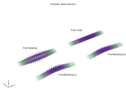
In the Settings window for 3D Plot Group, type Mode Shape, Clamped, Base Solution in the Label text field.
2
Click to expand the Title section. From the Title type list, choose Manual.
3
In the Title text area, type Clamped, Base Solution.
4
Clear the Parameter indicator text field.
5
Locate the Plot Settings section. Clear the Plot dataset edges checkbox.
6
Click to expand the Plot Array section. From the Array type list, choose Square.
7
In the Relative row padding text field, type 0.6.
8
In the Relative column padding text field, type 0.4.
First Bending, z Direction
1
In the Model Builder window, expand the Mode Shape, Clamped, Base Solution node, then click Surface 1.
2
In the Settings window for Surface, type First Bending, z Direction in the Label text field.
First Bending, y Direction
1
Right-click First Bending, z Direction and choose Duplicate.
2
In the Settings window for Surface, type First Bending, y Direction in the Label text field.
3
Locate the Data section. From the Dataset list, choose Study 1, Clamped, Base Solution/Solution 1 (sol1).
4
From the Eigenfrequency (Hz) list, choose 97660.
5
In the Mode Shape, Clamped, Base Solution toolbar, click  Plot.
6
Click the  Zoom Extents button in the Graphics toolbar.
First Twisting
1
Right-click First Bending, y Direction and choose Duplicate.
2
In the Settings window for Surface, locate the Data section.
3
From the Eigenfrequency (Hz) list, choose 2.669E5.
4
In the Label text field, type First Twisting.
5
In the Mode Shape, Clamped, Base Solution toolbar, click  Plot.
6
Click the  Zoom Extents button in the Graphics toolbar.
First Axial
1
Right-click First Twisting and choose Duplicate.
2
In the Settings window for Surface, type First Axial in the Label text field.
3
Locate the Data section. From the Eigenfrequency (Hz) list, choose 5E5.
4
In the Mode Shape, Clamped, Base Solution toolbar, click  Plot.
5
Click the  Zoom Extents button in the Graphics toolbar.
Deformation
1
In the Model Builder window, expand the Results > Mode Shape, Clamped, Base Solution > First Bending, z Direction node, then click Deformation.
2
In the Settings window for Deformation, locate the Scale section.
3
Select the Scale factor checkbox. In the associated text field, type 4E-4.
First Bending, y Direction
1
In the Model Builder window, under Results > Mode Shape, Clamped, Base Solution click First Bending, y Direction.
2
In the Settings window for Surface, click to expand the Inherit Style section.
3
From the Plot list, choose First Bending, z Direction.
First Twisting
1
In the Model Builder window, click First Twisting.
2
In the Settings window for Surface, locate the Inherit Style section.
3
From the Plot list, choose First Bending, z Direction.
First Axial
1
In the Model Builder window, click First Axial.
2
In the Settings window for Surface, locate the Inherit Style section.
3
From the Plot list, choose First Bending, z Direction.
4
In the Mode Shape, Clamped, Base Solution toolbar, click  Plot.
Arrow Surface, First Bending, z Direction
1
In the Model Builder window, right-click Mode Shape, Clamped, Base Solution and choose Arrow Surface.
2
In the Settings window for Arrow Surface, type Arrow Surface, First Bending, z Direction in the Label text field.
3
Locate the Arrow Positioning section. In the Number of arrows text field, type 100.
4
Locate the Coloring and Style section.
5
Select the Scale factor checkbox. In the associated text field, type 6E-4.
6
Click to expand the Plot Array section. Select the Manual indexing checkbox.
7
Locate the Coloring and Style section. From the Color list, choose Black.
Deformation 1
1
Right-click Arrow Surface, First Bending, z Direction and choose Deformation.
2
In the Settings window for Deformation, locate the Scale section.
3
Select the Scale factor checkbox. In the associated text field, type 4E-4.
4
In the Mode Shape, Clamped, Base Solution toolbar, click  Plot.
Results
Arrow Surface, First Bending, z Direction
In the Model Builder window, collapse the Results > Mode Shape, Clamped, Base Solution > Arrow Surface, First Bending, z Direction node.
Arrow Surface, First Bending, y Direction
1
In the Model Builder window, right-click Mode Shape, Clamped, Base Solution and choose Arrow Surface.
2
In the Settings window for Arrow Surface, type Arrow Surface, First Bending, y Direction in the Label text field.
3
Locate the Data section. From the Dataset list, choose Study 1, Clamped, Base Solution/Solution 1 (sol1).
4
From the Eigenfrequency (Hz) list, choose 97660.
5
Locate the Arrow Positioning section. In the Number of arrows text field, type 100.
6
Locate the Plot Array section. Select the Manual indexing checkbox.
7
In the Column index text field, type 1.
8
Click to expand the Inherit Style section. From the Plot list, choose Arrow Surface, First Bending, z Direction.
Deformation 1
Right-click Arrow Surface, First Bending, y Direction and choose Deformation.
Arrow Surface, First Bending, y Direction
In the Model Builder window, collapse the Results > Mode Shape, Clamped, Base Solution > Arrow Surface, First Bending, y Direction node.
Arrow Surface, First Twisting
1
Right-click Arrow Surface, First Bending, y Direction and choose Duplicate.
2
In the Settings window for Arrow Surface, type Arrow Surface, First Twisting in the Label text field.
3
Locate the Data section. From the Eigenfrequency (Hz) list, choose 2.669E5.
4
Locate the Plot Array section. In the Row index text field, type 1.
5
In the Column index text field, type 0.
6
In the Mode Shape, Clamped, Base Solution toolbar, click  Plot.
Arrow Surface, First Axial
1
Right-click Arrow Surface, First Twisting and choose Duplicate.
2
In the Settings window for Arrow Surface, locate the Data section.
3
From the Eigenfrequency (Hz) list, choose 5E5.
4
In the Label text field, type Arrow Surface, First Axial.
5
Locate the Plot Array section. In the Column index text field, type 1.
Transparency 1
In the Model Builder window, right-click First Bending, z Direction and choose Transparency.
Transparency 1
In the Model Builder window, right-click First Bending, y Direction and choose Transparency.
Transparency 1
In the Model Builder window, right-click First Twisting and choose Transparency.
Transparency 1
In the Model Builder window, right-click First Axial and choose Transparency.
First Bending, z Direction
In the Model Builder window, collapse the First Bending, z Direction node.
First Bending, y Direction
In the Model Builder window, collapse the Results > Mode Shape, Clamped, Base Solution > First Bending, y Direction node.
First Twisting
In the Model Builder window, collapse the Results > Mode Shape, Clamped, Base Solution > First Twisting node.
First Axial
In the Model Builder window, collapse the Results > Mode Shape, Clamped, Base Solution > First Axial node.
Mode Shape, Clamped, Base Solution
In the Model Builder window, click Mode Shape, Clamped, Base Solution.
Table Annotation 1
1
In the Mode Shape, Clamped, Base Solution toolbar, click  More Plots and choose Table Annotation.
2
In the Settings window for Table Annotation, locate the Data section.
3
From the Source list, choose Local table.
4
5
Locate the Coloring and Style section. Clear the Show point checkbox.
6
In the Mode Shape, Clamped, Base Solution toolbar, click  Plot.
7
Click the  Zoom Extents button in the Graphics toolbar.
8
Click the  Show Grid button in the Graphics toolbar.
Add a view for the plot
Definitions
View 2, 4 Beams
1
In the Model Builder window, under Component 1 (comp1) right-click Definitions and choose View.
2
In the Settings window for View, type View 2, 4 Beams in the Label text field.
Results
Mode Shape, Clamped, Base Solution
1
In the Model Builder window, under Results click Mode Shape, Clamped, Base Solution.
2
In the Settings window for 3D Plot Group, locate the Plot Settings section.
3
From the View list, choose View 2, 4 Beams.
Return to the default view to continue the modeling.
Solid Mechanics (solid)
Click the  Zoom Extents button in the Graphics toolbar.
Results
In the Model Builder window, collapse the Results > Mode Shape, Clamped, Base Solution node.
Evaluate eigenfrequencies.
Eigenfrequencies (Study 1, Clamped, Base Solution)
1
In the Model Builder window, click Eigenfrequencies (Study 1, Clamped, Base Solution).
2
In the Eigenfrequencies (Study 1, Clamped, Base Solution) toolbar, click  Evaluate.
Participation Factors (Study 1, Clamped, Base Solution)
1
In the Model Builder window, click Participation Factors (Study 1, Clamped, Base Solution).
2
In the Participation Factors (Study 1, Clamped, Base Solution) toolbar, click  Evaluate.
Add a study for the cantilever beam case.
Add Study
1
In the Study toolbar, click  Add Study to open the Add Study window.
2
Go to the Add Study window.
3
Find the Studies subsection. In the Select Study tree, select General Studies > Eigenfrequency.
4
Click the Add Study button in the window toolbar.
5
In the Study toolbar, click  Add Study to close the Add Study window.
Study 2
1
In the Settings window for Study, locate the Study Settings section.
2
Clear the Generate default plots checkbox.
Step 1: Eigenfrequency
1
In the Model Builder window, under Study 2 click Step 1: Eigenfrequency.
2
In the Settings window for Eigenfrequency, locate the Study Settings section.
3
Select the Desired number of eigenfrequencies checkbox. In the associated text field, type 10.
4
In the Search for eigenfrequencies around shift text field, type 10000[Hz].
5
Locate the Physics and Variables Selection section. Select the Modify model configuration for study step checkbox.
6
In the tree, select Component 1 (comp1) > Solid Mechanics (solid) > Linear Elastic Material 1 > Thermal Expansion 1.
7
Disable the fixed constraint at the right end of the beam to obtain a cantilever.
8
In the tree, select Component 1 (comp1) > Solid Mechanics (solid) > Fixed Constraint, Right End.
9
10
In the Model Builder window, click Study 2.
11
In the Settings window for Study, type Study 2, Cantilever, Base solution in the Label text field.
Solution 2 (sol2)
1
In the Study toolbar, click  Show Default Solver.
2
In the Model Builder window, expand the Solution 2 (sol2) node, then click Eigenvalue Solver 1.
3
In the Settings window for Eigenvalue Solver, locate the General section.
4
In the Relative tolerance text field, type 1.0E-30.
5
Locate the Output section. In the Maximum absolute value text field, type 1.
6
In the Study toolbar, click  Compute.
Results
Mode Shape, Cantilever, Base Solution
1
In the Model Builder window, right-click Mode Shape, Clamped, Base Solution and choose Duplicate.
2
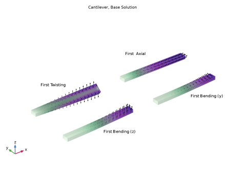
In the Settings window for 3D Plot Group, type Mode Shape, Cantilever, Base Solution in the Label text field.
3
Locate the Data section. From the Dataset list, choose Study 2, Cantilever, Base solution/Solution 2 (sol2).
4
Locate the Title section. In the Title text area, type Cantilever, Base Solution.
First Bending, y Direction
1
In the Model Builder window, expand the Mode Shape, Cantilever, Base Solution node, then click First Bending, y Direction.
2
In the Settings window for Surface, locate the Data section.
3
From the Dataset list, choose Study 2, Cantilever, Base solution/Solution 2 (sol2).
First Twisting
1
In the Model Builder window, click First Twisting.
2
In the Settings window for Surface, locate the Data section.
3
From the Dataset list, choose Study 2, Cantilever, Base solution/Solution 2 (sol2).
4
From the Eigenfrequency (Hz) list, choose 1.3223E5.
First Axial
1
In the Model Builder window, click First Axial.
2
In the Settings window for Surface, locate the Data section.
3
From the Dataset list, choose Study 2, Cantilever, Base solution/Solution 2 (sol2).
4
From the Eigenfrequency (Hz) list, choose 2.5E5.
Arrow Surface, First Bending, y Direction
1
In the Model Builder window, click Arrow Surface, First Bending, y Direction.
2
In the Settings window for Arrow Surface, locate the Data section.
3
From the Dataset list, choose Study 2, Cantilever, Base solution/Solution 2 (sol2).
Arrow Surface, First Twisting
1
In the Model Builder window, click Arrow Surface, First Twisting.
2
In the Settings window for Arrow Surface, locate the Data section.
3
From the Dataset list, choose Study 2, Cantilever, Base solution/Solution 2 (sol2).
4
From the Eigenfrequency (Hz) list, choose 1.3223E5.
Arrow Surface, First Axial
1
In the Model Builder window, click Arrow Surface, First Axial.
2
In the Settings window for Arrow Surface, locate the Data section.
3
From the Dataset list, choose Study 2, Cantilever, Base solution/Solution 2 (sol2).
4
From the Eigenfrequency (Hz) list, choose 2.5E5.
5
In the Mode Shape, Cantilever, Base Solution toolbar, click  Plot.
6
Click the  Show Grid button in the Graphics toolbar.
Results
Mode Shape, Cantilever, Base Solution
In the Model Builder window, collapse the Results > Mode Shape, Cantilever, Base Solution node.
Eigenfrequencies (Study 2, Cantilever, Base Solution)
1
In the Model Builder window, right-click Eigenfrequencies (Study 1, Clamped, Base Solution) and choose Duplicate.
2
In the Settings window for Evaluation Group, locate the Data section.
3
From the Dataset list, choose Study 2, Cantilever, Base solution/Solution 2 (sol2).
4
In the Label text field, type Eigenfrequencies (Study 2, Cantilever, Base Solution).
5
In the Eigenfrequencies (Study 2, Cantilever, Base Solution) toolbar, click  Evaluate.
Participation Factors (Study 2, Cantilever, Base Solution)
1
In the Model Builder window, right-click Participation Factors (Study 1, Clamped, Base Solution) and choose Duplicate.
2
In the Settings window for Evaluation Group, locate the Data section.
3
From the Dataset list, choose Study 2, Cantilever, Base solution/Solution 2 (sol2).
4
In the Label text field, type Participation Factors (Study 2, Cantilever, Base Solution).
5
In the Participation Factors (Study 2, Cantilever, Base Solution) toolbar, click  Evaluate.
Eigenfrequencies (Study 1, Clamped, Base Solution), Mode Shape, Clamped, Base Solution, Participation Factors (Study 1, Clamped, Base Solution)
1
In the Model Builder window, under Results, Ctrl-click to select Mode Shape, Clamped, Base Solution, Eigenfrequencies (Study 1, Clamped, Base Solution), and Participation Factors (Study 1, Clamped, Base Solution).
2
Clamped
In the Settings window for Group, type Clamped in the Label text field.
Eigenfrequencies (Study 1, Clamped, Base Solution)
In the Model Builder window, collapse the Results > Clamped > Eigenfrequencies (Study 1, Clamped, Base Solution) node.
Participation Factors (Study 1, Clamped, Base Solution)
In the Model Builder window, collapse the Results > Clamped > Participation Factors (Study 1, Clamped, Base Solution) node.
Mode Shape, Clamped, Base Solution
In the Model Builder window, collapse the Results > Clamped > Mode Shape, Clamped, Base Solution node.
Clamped
In the Model Builder window, collapse the Results > Clamped node.
Eigenfrequencies (Study 2, Cantilever, Base Solution), Mode Shape, Cantilever, Base Solution, Participation Factors (Study 2, Cantilever, Base Solution)
1
In the Model Builder window, under Results, Ctrl-click to select Mode Shape, Cantilever, Base Solution, Eigenfrequencies (Study 2, Cantilever, Base Solution), and Participation Factors (Study 2, Cantilever, Base Solution).
2
Cantilever
In the Settings window for Group, type Cantilever in the Label text field.
Mode Shape, Cantilever, Base Solution
In the Model Builder window, collapse the Results > Cantilever > Mode Shape, Cantilever, Base Solution node.
Eigenfrequencies (Study 2, Cantilever, Base Solution)
In the Model Builder window, collapse the Results > Cantilever > Eigenfrequencies (Study 2, Cantilever, Base Solution) node.
Participation Factors (Study 2, Cantilever, Base Solution)
In the Model Builder window, collapse the Results > Cantilever > Participation Factors (Study 2, Cantilever, Base Solution) node.
Cantilever
In the Model Builder window, collapse the Results > Cantilever node.
Now, analyze the effect of a temperature shift.
Add Study
1
In the Study toolbar, click  Add Study to open the Add Study window.
2
Go to the Add Study window.
3
Find the Studies subsection. In the Select Study tree, select Preset Studies for Selected Physics Interfaces > Eigenfrequency, Prestressed.
4
Click the Add Study button in the window toolbar.
Study 3, Clamped, dT
1
In the Settings window for Study, type Study 3, Clamped, dT in the Label text field.
2
Locate the Study Settings section. Clear the Generate default plots checkbox.
In this case, it would be possible to use a geometrically linear study.
Step 1: Stationary
1
In the Model Builder window, under Study 3, Clamped, dT click Step 1: Stationary.
2
In the Settings window for Stationary, locate the Study Settings section.
3
Clear the Include geometric nonlinearity checkbox.
Step 2: Eigenfrequency
1
In the Model Builder window, click Step 2: Eigenfrequency.
2
In the Settings window for Eigenfrequency, locate the Study Settings section.
3
Select the Desired number of eigenfrequencies checkbox. In the associated text field, type 10.
4
In the Search for eigenfrequencies around shift text field, type 10000[Hz].
Parametric Sweep
1
In the Study toolbar, click  Parametric Sweep.
2
In the Settings window for Parametric Sweep, locate the Study Settings section.
3
4
5
Click  Range.
6
In the Range dialog, type 0 in the Start text field.
7
In the Step text field, type 2.
8
In the Stop text field, type 10.
9
Click Add.
Solution 3 (sol3)
In the Study toolbar, click  Show Default Solver.
Solution 3 (sol3)
1
In the Model Builder window, expand the Study 3, Clamped, dT > Solver Configurations > Solution 3 (sol3) node, then click Eigenvalue Solver 1.
2
In the Settings window for Eigenvalue Solver, locate the General section.
3
In the Relative tolerance text field, type 1.0E-30.
4
Locate the Output section. From the Scaling of eigenvectors list, choose RMS.
Study 3, Clamped, dT
1
In the Model Builder window, collapse the Study 3, Clamped, dT > Solver Configurations > Solution 3 (sol3) node.
2
In the Study toolbar, click  Add Study to close the Add Study window.
3
In the Study toolbar, click  Compute.
Plot the frequency shift as a function of the temperature variation.
Results
Frequency Shift with Temperature, Clamped
1
In the Results toolbar, click  1D Plot Group.
2
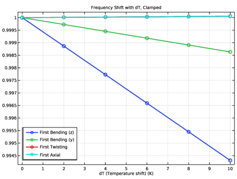
In the Settings window for 1D Plot Group, type Frequency Shift with Temperature, Clamped in the Label text field.
3
Locate the Data section. From the Dataset list, choose Study 3, Clamped, dT/Parametric Solutions 1 (sol5).
4
From the Eigenfrequency selection list, choose First.
5
Click to expand the Title section. From the Title type list, choose Manual.
6
In the Title text area, type Frequency Shift with dT, Clamped.
First Bending Mode, z Direction
1
Right-click Frequency Shift with Temperature, Clamped and choose Global.
2
In the Settings window for Global, type First Bending Mode, z Direction in the Label text field.
3
Locate the y-Axis Data section. In the table, enter the following settings:
4
Locate the x-Axis Data section. From the Axis source data list, choose Outer solutions.
5
Click to expand the Coloring and Style section. From the Width list, choose 2.
6
Find the Line markers subsection. From the Marker list, choose Circle.
7
Click to expand the Legends section. From the Legends list, choose Manual.
8
9
In the Frequency Shift with Temperature, Clamped toolbar, click  Plot.
First Bending Mode, y Direction
1
Right-click First Bending Mode, z Direction and choose Duplicate.
2
In the Settings window for Global, type First Bending Mode, y Direction in the Label text field.
3
Locate the Data section. From the Dataset list, choose Study 3, Clamped, dT/Parametric Solutions 1 (sol5).
4
From the Eigenfrequency selection list, choose Manual.
5
In the Eigenfrequency indices (1-10) text field, type 2.
6
Locate the y-Axis Data section. In the table, enter the following settings:
7
Locate the Legends section. In the table, enter the following settings:
8
In the Frequency Shift with Temperature, Clamped toolbar, click  Plot.
First Twisting Mode
1
Right-click First Bending Mode, y Direction and choose Duplicate.
2
In the Settings window for Global, type First Twisting Mode in the Label text field.
3
Locate the Data section. In the Eigenfrequency indices (1-10) text field, type 6.
4
Locate the y-Axis Data section. In the table, enter the following settings:
5
Locate the Legends section. In the table, enter the following settings:
6
In the Frequency Shift with Temperature, Clamped toolbar, click  Plot.
First Axial Mode
1
Right-click First Twisting Mode and choose Duplicate.
2
In the Settings window for Global, type First Axial Mode in the Label text field.
3
Locate the Data section. In the Eigenfrequency indices (1-10) text field, type 9.
4
Locate the y-Axis Data section. In the table, enter the following settings:
5
Locate the Legends section. In the table, enter the following settings:
6
In the Frequency Shift with Temperature, Clamped toolbar, click  Plot.
Frequency Shift with Temperature, Clamped
1
In the Model Builder window, click Frequency Shift with Temperature, Clamped.
2
In the Settings window for 1D Plot Group, locate the Legend section.
3
From the Position list, choose Lower left.
4
In the Frequency Shift with Temperature, Clamped toolbar, click  Plot.
Repeat for the cantilever.
Add Study
1
In the Home toolbar, click  Add Study to open the Add Study window.
2
Go to the Add Study window.
3
Find the Studies subsection. In the Select Study tree, select Preset Studies for Selected Physics Interfaces > Eigenfrequency, Prestressed.
4
Click the Add Study button in the window toolbar.
5
In the Home toolbar, click  Add Study to close the Add Study window.
Study 4, Cantilever, dT
1
In the Settings window for Study, type Study 4, Cantilever, dT in the Label text field.
2
Locate the Study Settings section. Clear the Generate default plots checkbox.
Step 1: Stationary
1
In the Model Builder window, under Study 4, Cantilever, dT click Step 1: Stationary.
2
In the Settings window for Stationary, locate the Study Settings section.
3
Clear the Include geometric nonlinearity checkbox.
4
Locate the Physics and Variables Selection section. Select the Modify model configuration for study step checkbox.
5
In the tree, select Component 1 (comp1) > Solid Mechanics (solid) > Fixed Constraint, Right End.
6
Step 2: Eigenfrequency
1
In the Model Builder window, click Step 2: Eigenfrequency.
2
In the Settings window for Eigenfrequency, locate the Study Settings section.
3
Select the Desired number of eigenfrequencies checkbox. In the associated text field, type 10.
4
In the Search for eigenfrequencies around shift text field, type 10000[Hz].
5
Locate the Physics and Variables Selection section. Select the Modify model configuration for study step checkbox.
6
In the tree, select Component 1 (comp1) > Solid Mechanics (solid), Controls spatial frame > Fixed Constraint, Right End.
7
Parametric Sweep
1
In the Study toolbar, click  Parametric Sweep.
2
In the Settings window for Parametric Sweep, locate the Study Settings section.
3
4
5
Click  Range.
6
In the Range dialog, type 0 in the Start text field.
7
In the Step text field, type 2.
8
In the Stop text field, type 10.
9
Click Add.
Solution 12 (sol12)
1
In the Study toolbar, click  Show Default Solver.
2
In the Model Builder window, expand the Solution 12 (sol12) node, then click Eigenvalue Solver 1.
3
In the Settings window for Eigenvalue Solver, locate the General section.
4
In the Relative tolerance text field, type 1.0E-30.
5
Locate the Output section. From the Scaling of eigenvectors list, choose RMS.
Study 4, Cantilever, dT
1
In the Model Builder window, collapse the Study 4, Cantilever, dT > Solver Configurations > Solution 12 (sol12) node.
2
In the Study toolbar, click  Compute.
Results
Frequency Shift with Temperature, Cantilever
1
In the Model Builder window, right-click Frequency Shift with Temperature, Clamped and choose Duplicate.
2
In the Settings window for 1D Plot Group, type Frequency Shift with Temperature, Cantilever in the Label text field.
3
Locate the Data section. From the Dataset list, choose Study 4, Cantilever, dT/Parametric Solutions 2 (sol14).
4
Locate the Title section. In the Title text area, type Frequency Shift with dT, Cantilever.
First Bending Mode, z Direction
1
In the Model Builder window, expand the Frequency Shift with Temperature, Cantilever node, then click First Bending Mode, z Direction.
2
In the Settings window for Global, locate the y-Axis Data section.
3
First Bending Mode, y Direction
1
In the Model Builder window, click First Bending Mode, y Direction.
2
In the Settings window for Global, locate the Data section.
3
From the Dataset list, choose Study 4, Cantilever, dT/Parametric Solutions 2 (sol14).
4
Locate the y-Axis Data section. In the table, enter the following settings:
First Twisting Mode
1
In the Model Builder window, click First Twisting Mode.
2
In the Settings window for Global, locate the Data section.
3
From the Dataset list, choose Study 4, Cantilever, dT/Parametric Solutions 2 (sol14).
4
In the Eigenfrequency indices (1-10) text field, type 5.
5
Locate the y-Axis Data section. In the table, enter the following settings:
First Axial Mode
1
In the Model Builder window, click First Axial Mode.
2
In the Settings window for Global, locate the Data section.
3
From the Dataset list, choose Study 4, Cantilever, dT/Parametric Solutions 2 (sol14).
4
In the Eigenfrequency indices (1-10) text field, type 7.
5
Locate the y-Axis Data section. In the table, enter the following settings:
6
In the Frequency Shift with Temperature, Cantilever toolbar, click  Plot.
Frequency Shift with Temperature, Cantilever
1
In the Model Builder window, click Frequency Shift with Temperature, Cantilever.
2
In the Settings window for 1D Plot Group, locate the Legend section.
3
From the Position list, choose Upper left.
4
In the Frequency Shift with Temperature, Cantilever toolbar, click  Plot.
5
In the Model Builder window, collapse the Frequency Shift with Temperature, Cantilever node.
Frequency Shift with Temperature, Clamped
1
In the Model Builder window, expand the Results > Clamped node, then click Frequency Shift with Temperature, Clamped.
2
Drag and drop below Clamped > Mode Shape, Clamped, Base Solution.
Frequency Shift with Temperature, Cantilever
1
In the Model Builder window, expand the Results > Cantilever node, then click Frequency Shift with Temperature, Cantilever.
2
Drag and drop below Cantilever > Mode Shape, Cantilever, Base Solution.
Frequency Shift with Temperature, Clamped
1
In the Results toolbar, click  Evaluation Group.
2
In the Settings window for Evaluation Group, type Frequency Shift with Temperature, Clamped in the Label text field.
3
Locate the Data section. From the Dataset list, choose Study 3, Clamped, dT/Parametric Solutions 1 (sol5).
4
Click to expand the Format section. From the Concatenation list, choose Vertical.
First Bending (z)
1
Right-click Frequency Shift with Temperature, Clamped and choose Global Evaluation.
2
In the Settings window for Global Evaluation, locate the Data section.
3
From the Dataset list, choose Study 3, Clamped, dT/Parametric Solutions 1 (sol5).
4
From the Eigenfrequency selection list, choose First.
5
Locate the Expressions section. In the table, enter the following settings:
6
Locate the Data section. From the Parameter selection (dT) list, choose Last.
7
In the Label text field, type First Bending (z).
First Bending (y)
1
Right-click First Bending (z) and choose Duplicate.
2
In the Settings window for Global Evaluation, type First Bending (y) in the Label text field.
3
Locate the Data section. From the Eigenfrequency selection list, choose Manual.
4
In the Eigenfrequency indices (1-10) text field, type 2.
5
Locate the Expressions section. In the table, enter the following settings:
First Twisting
1
Right-click First Bending (y) and choose Duplicate.
2
In the Settings window for Global Evaluation, type First Twisting in the Label text field.
3
Locate the Data section. In the Eigenfrequency indices (1-10) text field, type 6.
4
Locate the Expressions section. In the table, enter the following settings:
First Axial
1
Right-click First Twisting and choose Duplicate.
2
In the Settings window for Global Evaluation, locate the Data section.
3
In the Eigenfrequency indices (1-10) text field, type 9.
4
Locate the Expressions section. In the table, enter the following settings:
5
In the Label text field, type First Axial.
6
In the Frequency Shift with Temperature, Clamped toolbar, click  Evaluate.
Frequency Shift with Temperature, Clamped
In the Model Builder window, right-click Frequency Shift with Temperature, Clamped and choose Copy.
Frequency Shift with Temperature, Cantilever
1
In the Model Builder window, right-click Cantilever and choose Paste Evaluation Group.
2
In the Settings window for Evaluation Group, type Frequency Shift with Temperature, Cantilever in the Label text field.
3
Locate the Data section. From the Dataset list, choose Study 4, Cantilever, dT/Parametric Solutions 2 (sol14).
First Bending (z)
1
In the Model Builder window, expand the Frequency Shift with Temperature, Cantilever node, then click First Bending (z).
2
In the Settings window for Global Evaluation, locate the Data section.
3
From the Dataset list, choose Study 4, Cantilever, dT/Parametric Solutions 2 (sol14).
4
Locate the Expressions section. In the table, enter the following settings:
First Bending (y)
1
In the Model Builder window, click First Bending (y).
2
In the Settings window for Global Evaluation, locate the Data section.
3
From the Dataset list, choose Study 4, Cantilever, dT/Parametric Solutions 2 (sol14).
4
Locate the Expressions section. In the table, enter the following settings:
First Twisting
1
In the Model Builder window, click First Twisting.
2
In the Settings window for Global Evaluation, locate the Data section.
3
From the Dataset list, choose Study 4, Cantilever, dT/Parametric Solutions 2 (sol14).
4
In the Eigenfrequency indices (1-10) text field, type 5.
5
Locate the Expressions section. In the table, enter the following settings:
First Axial
1
In the Model Builder window, click First Axial.
2
In the Settings window for Global Evaluation, locate the Data section.
3
From the Dataset list, choose Study 4, Cantilever, dT/Parametric Solutions 2 (sol14).
4
In the Eigenfrequency indices (1-10) text field, type 7.
5
Locate the Expressions section. In the table, enter the following settings:
6
In the Frequency Shift with Temperature, Cantilever toolbar, click  Evaluate.
Frequency Shift with Temperature, Cantilever
In the Model Builder window, collapse the Results > Cantilever > Frequency Shift with Temperature, Cantilever node.
Frequency Shift with Temperature, Clamped
In the Model Builder window, collapse the Results > Clamped > Frequency Shift with Temperature, Clamped node.
Compute the buckling critical load for the clamped case.
Add Study
1
In the Study toolbar, click  Add Study to open the Add Study window.
2
Go to the Add Study window.
3
Find the Studies subsection. In the Select Study tree, select Preset Studies for Selected Physics Interfaces > Linear Buckling.
4
Click the Add Study button in the window toolbar.
5
In the Study toolbar, click  Add Study to close the Add Study window.
Study 5, Buckling
In the Settings window for Study, type Study 5, Buckling in the Label text field.
Step 2: Linear Buckling
In the Study toolbar, click  Compute.
Results
Mode Shape, Buckling
1
In the Settings window for 3D Plot Group, type Mode Shape, Buckling in the Label text field.
2
Drag and drop below Clamped > Frequency Shift with Temperature, Clamped.
3
Click the  Zoom Extents button in the Graphics toolbar.
Add a view for the buckling plot.
Definitions
View 3: Buckling
1
In the Model Builder window, under Component 1 (comp1) right-click Definitions and choose View.
2
In the Settings window for View, type View 3: Buckling in the Label text field.
Results
Mode Shape, Buckling
1
In the Model Builder window, under Results > Clamped click Mode Shape, Buckling.
2
In the Settings window for 3D Plot Group, locate the Plot Settings section.
3
From the View list, choose View 3: Buckling.
Return to the default view to continue the modeling.
Definitions
View 1
Compare the numerical results obtained for the cantilever with the estimated expected shifts.
Variables 1
1
In the Model Builder window, right-click Definitions and choose Variables.
2
In the Settings window for Variables, locate the Variables section.
3
Study 4, Cantilever, dT
In the Study toolbar, click  Update Solution.
Results
First Bending (z)
1
In the Model Builder window, under Results > Cantilever > Frequency Shift with Temperature, Cantilever click First Bending (z).
2
In the Settings window for Global Evaluation, locate the Expressions section.
3
First Bending (y)
1
In the Model Builder window, click First Bending (y).
2
In the Settings window for Global Evaluation, locate the Expressions section.
3
First Twisting
1
In the Model Builder window, click First Twisting.
2
In the Settings window for Global Evaluation, locate the Expressions section.
3
First Axial
1
In the Model Builder window, click First Axial.
2
In the Settings window for Global Evaluation, locate the Expressions section.
3
4
In the Frequency Shift with Temperature, Cantilever toolbar, click  Evaluate.
Frequency Shift with Temperature, Cantilever
1
Go to the Frequency Shift with Temperature, Cantilever window.
2
Click the Full Precision button in the window toolbar to better compare numerical results with estimates.
3
Click the Full Precision button in the window toolbar to revert to the default precision.
Add plots of the estimates of the frequency shift versus temperature to get a visual comparison with the numerical results.
Results
Frequency Shift with Temperature, Cantilever
In the Model Builder window, expand the Frequency Shift with Temperature, Cantilever node.
First Axial Mode, First Bending Mode, y Direction, First Bending Mode, z Direction, First Twisting Mode
1
In the Model Builder window, under Results > Cantilever > Frequency Shift with Temperature, Cantilever, Ctrl-click to select First Bending Mode, z Direction, First Bending Mode, y Direction, First Twisting Mode, and First Axial Mode.
2
First Bending Mode, z Direction (Estimate)
1
In the Settings window for Global, type First Bending Mode, z Direction (Estimate) in the Label text field.
2
Locate the y-Axis Data section. In the table, enter the following settings:
3
Locate the Coloring and Style section. Find the Line style subsection. From the Line list, choose Dashed.
4
Find the Line markers subsection. From the Marker list, choose Square.
5
Locate the Legends section. In the table, enter the following settings:
First Bending Mode, y Direction (Estimate)
1
In the Model Builder window, under Results > Cantilever > Frequency Shift with Temperature, Cantilever click First Bending Mode, y Direction 1.
2
In the Settings window for Global, type First Bending Mode, y Direction (Estimate) in the Label text field.
3
Locate the y-Axis Data section. In the table, enter the following settings:
4
Locate the Coloring and Style section. Find the Line style subsection. From the Line list, choose Dashed.
5
Find the Line markers subsection. From the Marker list, choose Square.
6
Locate the Legends section. In the table, enter the following settings:
First Twisting Mode (Estimate)
1
In the Model Builder window, under Results > Cantilever > Frequency Shift with Temperature, Cantilever click First Twisting Mode 1.
2
In the Settings window for Global, type First Twisting Mode (Estimate) in the Label text field.
3
Locate the y-Axis Data section. In the table, enter the following settings:
4
Locate the Coloring and Style section. Find the Line style subsection. From the Line list, choose Dashed.
5
Find the Line markers subsection. From the Marker list, choose Square.
6
Locate the Legends section. In the table, enter the following settings:
First Axial Mode (Estimate)
1
In the Model Builder window, under Results > Cantilever > Frequency Shift with Temperature, Cantilever click First Axial Mode 1.
2
In the Settings window for Global, type First Axial Mode (Estimate) in the Label text field.
3
Locate the y-Axis Data section. In the table, enter the following settings:
4
Locate the Coloring and Style section. Find the Line style subsection. From the Line list, choose Dashed.
5
Find the Line markers subsection. From the Marker list, choose Square.
6
Locate the Legends section. In the table, enter the following settings:
First Bending Mode, z Direction (Estimate)
1
In the Model Builder window, click First Bending Mode, z Direction (Estimate).
2
In the Settings window for Global, locate the Coloring and Style section.
3
From the Color list, choose Cycle (reset).
Frequency Shift with Temperature, Cantilever
In the Model Builder window, collapse the Results > Cantilever > Frequency Shift with Temperature, Cantilever node.
Inspect stress concentration at the fixed boundary.
Stress at Clamp
1
In the Results toolbar, click  3D Plot Group.
2
In the Settings window for 3D Plot Group, type Stress at Clamp in the Label text field.
3
Locate the Data section. From the Dataset list, choose Study 4, Cantilever, dT/Solution Store 2 (sol13).
Volume 1
1
Right-click Stress at Clamp and choose Volume.
2
In the Settings window for Volume, locate the Expression section.
3
In the Expression text field, type solid.sx.
4
In the Stress at Clamp toolbar, click  Plot.
5
From the Unit list, choose MPa.
6
Locate the Coloring and Style section. From the Color table list, choose Rainbow.
Introduce thermal expansion of constraints.
Solid Mechanics (solid)
Fixed Constraint, Left End
In the Model Builder window, under Component 1 (comp1) > Solid Mechanics (solid) click Fixed Constraint, Left End.
Thermal Expansion 1
1
In the Physics toolbar, click  Attributes and choose Thermal Expansion.
2
In the Settings window for Thermal Expansion, locate the Thermal Expansion Properties section.
3
Select the Inherit from domain checkbox.
Modify the previous studies for future reruns to not include the constraint thermal expansion.
Study 1, Clamped, Base Solution
Step 1: Eigenfrequency
1
In the Model Builder window, under Study 1, Clamped, Base Solution click Step 1: Eigenfrequency.
2
In the Settings window for Eigenfrequency, locate the Physics and Variables Selection section.
3
In the tree, select Component 1 (comp1) > Solid Mechanics (solid) > Fixed Constraint, Left End > Thermal Expansion 1.
4
Study 2, Cantilever, Base solution
1
In the Model Builder window, under Study 2, Cantilever, Base solution click Step 1: Eigenfrequency.
2
In the Settings window for Eigenfrequency, locate the Physics and Variables Selection section.
3
Study 3, Clamped, dT
Step 1: Stationary
1
In the Model Builder window, under Study 3, Clamped, dT click Step 1: Stationary.
2
In the Settings window for Stationary, locate the Physics and Variables Selection section.
3
Select the Modify model configuration for study step checkbox.
4
In the tree, select Component 1 (comp1) > Solid Mechanics (solid) > Fixed Constraint, Left End > Thermal Expansion 1.
5
Step 2: Eigenfrequency
1
In the Model Builder window, click Step 2: Eigenfrequency.
2
In the Settings window for Eigenfrequency, locate the Physics and Variables Selection section.
3
Select the Modify model configuration for study step checkbox.
4
Study 4, Cantilever, dT
Step 1: Stationary
1
In the Model Builder window, under Study 4, Cantilever, dT click Step 1: Stationary.
2
In the Settings window for Stationary, locate the Physics and Variables Selection section.
3
Step 2: Eigenfrequency
1
In the Model Builder window, click Step 2: Eigenfrequency.
2
In the Settings window for Eigenfrequency, locate the Physics and Variables Selection section.
3
Study 5, Buckling
Step 1: Stationary
1
In the Model Builder window, under Study 5, Buckling click Step 1: Stationary.
2
In the Settings window for Stationary, locate the Physics and Variables Selection section.
3
Select the Modify model configuration for study step checkbox.
4
Step 2: Linear Buckling
1
In the Model Builder window, click Step 2: Linear Buckling.
2
In the Settings window for Linear Buckling, locate the Physics and Variables Selection section.
3
Select the Modify model configuration for study step checkbox.
4
In the tree, select Component 1 (comp1) > Solid Mechanics (solid) > Fixed Constraint, Left End > Thermal Expansion 1.
5
Study 1, Clamped, Base Solution
In the Model Builder window, collapse the Study 1, Clamped, Base Solution node.
Study 2, Cantilever, Base solution
In the Model Builder window, collapse the Study 2, Cantilever, Base solution node.
Study 3, Clamped, dT
In the Model Builder window, collapse the Study 3, Clamped, dT node.
Study 4, Cantilever, dT
In the Model Builder window, collapse the Study 4, Cantilever, dT node.
Study 5, Buckling
In the Model Builder window, collapse the Study 5, Buckling node.
Add Study
1
In the Home toolbar, click  Add Study to open the Add Study window.
2
Go to the Add Study window.
3
Find the Studies subsection. In the Select Study tree, select Preset Studies for Selected Physics Interfaces > Eigenfrequency, Prestressed.
4
Click the Add Study button in the window toolbar.
5
In the Home toolbar, click  Add Study to close the Add Study window.
Study 6, Cantilever with Expanding Constraint
1
In the Settings window for Study, type Study 6, Cantilever with Expanding Constraint in the Label text field.
2
Locate the Study Settings section. Clear the Generate default plots checkbox.
Step 1: Stationary
1
In the Model Builder window, under Study 6, Cantilever with Expanding Constraint click Step 1: Stationary.
2
In the Settings window for Stationary, locate the Physics and Variables Selection section.
3
Select the Modify model configuration for study step checkbox.
4
In the tree, select Component 1 (comp1) > Solid Mechanics (solid), Controls spatial frame > Fixed Constraint, Right End.
5
Step 2: Eigenfrequency
1
In the Model Builder window, click Step 2: Eigenfrequency.
2
In the Settings window for Eigenfrequency, locate the Study Settings section.
3
Select the Desired number of eigenfrequencies checkbox. In the associated text field, type 10.
4
In the Search for eigenfrequencies around shift text field, type 10000[Hz].
5
Locate the Physics and Variables Selection section. Select the Modify model configuration for study step checkbox.
6
In the tree, select Component 1 (comp1) > Solid Mechanics (solid), Controls spatial frame > Fixed Constraint, Right End.
7
Parametric Sweep
1
In the Study toolbar, click  Parametric Sweep.
2
In the Settings window for Parametric Sweep, locate the Study Settings section.
3
4
Solution 23 (sol23)
1
In the Study toolbar, click  Show Default Solver.
2
In the Model Builder window, expand the Solution 23 (sol23) node, then click Eigenvalue Solver 1.
3
In the Settings window for Eigenvalue Solver, locate the General section.
4
In the Relative tolerance text field, type 1.0E-30.
5
Locate the Output section. From the Scaling of eigenvectors list, choose RMS.
6
In the Study toolbar, click  Compute.
Results
Frequency Shift with Temperature, Cantilever, Expanding Constraint
1
In the Model Builder window, right-click Frequency Shift with Temperature, Cantilever and choose Duplicate.
2
In the Settings window for 1D Plot Group, type Frequency Shift with Temperature, Cantilever, Expanding Constraint in the Label text field.
3
Locate the Data section. From the Dataset list, choose Study 6, Cantilever with Expanding Constraint/Parametric Solutions 3 (sol25).
First Bending Mode, y Direction
1
In the Model Builder window, expand the Frequency Shift with Temperature, Cantilever, Expanding Constraint node, then click First Bending Mode, y Direction.
2
In the Settings window for Global, locate the Data section.
3
From the Dataset list, choose Study 6, Cantilever with Expanding Constraint/Parametric Solutions 3 (sol25).
First Twisting Mode
1
In the Model Builder window, click First Twisting Mode.
2
In the Settings window for Global, locate the Data section.
3
From the Dataset list, choose Study 6, Cantilever with Expanding Constraint/Parametric Solutions 3 (sol25).
First Axial Mode
1
In the Model Builder window, click First Axial Mode.
2
In the Settings window for Global, locate the Data section.
3
From the Dataset list, choose Study 6, Cantilever with Expanding Constraint/Parametric Solutions 3 (sol25).
4
In the Frequency Shift with Temperature, Cantilever, Expanding Constraint toolbar, click  Plot.
First Bending (z)
1
In the Model Builder window, under Results > Cantilever > Frequency Shift with Temperature, Cantilever click First Bending (z).
2
In the Settings window for Global Evaluation, locate the Expressions section.
3
First Bending (y)
1
In the Model Builder window, click First Bending (y).
2
In the Settings window for Global Evaluation, locate the Expressions section.
3
First Twisting
1
In the Model Builder window, click First Twisting.
2
In the Settings window for Global Evaluation, locate the Expressions section.
3
First Axial
1
In the Model Builder window, click First Axial.
2
In the Settings window for Global Evaluation, locate the Expressions section.
3
4
In the Frequency Shift with Temperature, Cantilever toolbar, click  Evaluate.
Compare the stress at the fixed boundary with that obtained without thermal expansion in the clamp.
Volume 2
1
In the Model Builder window, under Results > Cantilever > Stress at Clamp right-click Volume 1 and choose Duplicate.
2
In the Settings window for Volume, locate the Data section.
3
From the Dataset list, choose Study 6, Cantilever with Expanding Constraint/Solution Store 4 (sol24).
4
Click to expand the Inherit Style section. From the Plot list, choose Volume 1.
Stress at Clamp
1
In the Model Builder window, click Stress at Clamp.
2
In the Settings window for 3D Plot Group, locate the Plot Array section.
3
From the Array type list, choose Linear.
4
From the Array axis list, choose y.
5
In the Relative padding text field, type 5.
6
In the Stress at Clamp toolbar, click  Plot.
7
Locate the Title section. From the Title type list, choose Manual.
8
In the Title text area, type Stress tensor, x-component (MPa).
9
In the Stress at Clamp toolbar, click  Plot.
No Expanding Boundaries
1
In the Model Builder window, under Results > Cantilever > Stress at Clamp click Volume 1.
2
In the Settings window for Volume, type No Expanding Boundaries in the Label text field.
Expanding Boundaries
1
In the Model Builder window, under Results > Cantilever > Stress at Clamp click Volume 2.
2
In the Settings window for Volume, type Expanding Boundaries in the Label text field.
Deformation 1
In the Model Builder window, right-click No Expanding Boundaries and choose Deformation.
Deformation 1
In the Model Builder window, right-click Expanding Boundaries and choose Deformation.
Table Annotation 1
1
In the Stress at Clamp toolbar, click  More Plots and choose Table Annotation.
2
In the Settings window for Table Annotation, locate the Data section.
3
From the Source list, choose Local table.
4
5
Locate the Coloring and Style section. Clear the Show point checkbox.
6
From the Anchor point list, choose Lower left.
7
In the Stress at Clamp toolbar, click  Plot.
8
Click the  Zoom Extents button in the Graphics toolbar.
Definitions
View 4: 2 Beams
1
In the Model Builder window, under Component 1 (comp1) right-click Definitions and choose View.
2
In the Settings window for View, type View 4: 2 Beams in the Label text field.
Results
Stress at Clamp
1
In the Model Builder window, under Results > Cantilever click Stress at Clamp.
2
In the Settings window for 3D Plot Group, locate the Plot Settings section.
3
From the View list, choose View 4: 2 Beams.
Results
Expanding Boundaries
In the Model Builder window, collapse the Results > Cantilever > Stress at Clamp > Expanding Boundaries node.
No Expanding Boundaries
In the Model Builder window, collapse the Results > Cantilever > Stress at Clamp > No Expanding Boundaries node.
Frequency Shift with Temperature, Cantilever
In the Model Builder window, collapse the Results > Cantilever > Frequency Shift with Temperature, Cantilever node.
Stress at Clamp
In the Model Builder window, collapse the Results > Cantilever > Stress at Clamp node.
Frequency Shift with Temperature, Cantilever, Expanding Constraint
In the Model Builder window, collapse the Results > Cantilever > Frequency Shift with Temperature, Cantilever, Expanding Constraint node.
Clamped
In the Model Builder window, collapse the Results > Clamped node.
Study 1, Clamped, Base Solution
Solver Configurations
In the Model Builder window, collapse the Study 1, Clamped, Base Solution > Solver Configurations node.
Now, analyze the effect of a temperature dependent Young’s modulus.
Global Definitions
Material Properties
1
In the Model Builder window, under Global Definitions click Material Properties.
2
In the Settings window for Parameters, locate the Parameters section.
3
Materials
Material 1 (mat1)
1
In the Model Builder window, expand the Component 1 (comp1) > Materials > Material 1 (mat1) node, then click Basic (def).
2
In the Settings window for Basic, locate the Model Inputs section.
3
Click  Select Quantity.
4
In the Physical Quantity dialog, type Temperature in the text field.
5
In the tree, select General > Temperature (K).
6
7
In the Model Builder window, under Component 1 (comp1) > Materials > Material 1 (mat1) click Young’s modulus and Poisson’s ratio (Enu).
8
In the Settings window for Young’s Modulus and Poisson’s Ratio, locate the Model Inputs section.
9
Click  Select Quantity.
10
In the Physical Quantity dialog, select General > Temperature (K) in the tree.
11
12
In the Model Builder window, click Material 1 (mat1).
13
In the Settings window for Material, locate the Material Contents section.
14
Solid Mechanics (solid)
Linear Elastic Material 1
1
In the Model Builder window, under Component 1 (comp1) > Solid Mechanics (solid) click Linear Elastic Material 1.
2
In the Settings window for Linear Elastic Material, locate the Model Input section.
3
From the Tref list, choose User defined. From the T list, choose User defined. In the associated text field, type 293.15[K]+dT.
Add Study
1
In the Home toolbar, click  Add Study to open the Add Study window.
2
Go to the Add Study window.
3
Find the Studies subsection. In the Select Study tree, select Preset Studies for Selected Physics Interfaces > Eigenfrequency, Prestressed.
4
Click the Add Study button in the window toolbar.
5
In the Home toolbar, click  Add Study to close the Add Study window.
Study 7, Cantilever with Temperature Dependent E
1
In the Settings window for Study, type Study 7, Cantilever with Temperature Dependent E in the Label text field.
2
Locate the Study Settings section. Clear the Generate default plots checkbox.
Step 1: Stationary
1
In the Model Builder window, under Study 7, Cantilever with Temperature Dependent E click Step 1: Stationary.
2
In the Settings window for Stationary, locate the Study Settings section.
3
Clear the Include geometric nonlinearity checkbox.
4
Locate the Physics and Variables Selection section. Select the Modify model configuration for study step checkbox.
5
In the tree, select Component 1 (comp1) > Solid Mechanics (solid) > Fixed Constraint, Right End.
6
Step 2: Eigenfrequency
1
In the Model Builder window, click Step 2: Eigenfrequency.
2
In the Settings window for Eigenfrequency, locate the Study Settings section.
3
Select the Desired number of eigenfrequencies checkbox. In the associated text field, type 10.
4
In the Search for eigenfrequencies around shift text field, type 10000[Hz].
5
Locate the Physics and Variables Selection section. Select the Modify model configuration for study step checkbox.
6
In the tree, select Component 1 (comp1) > Solid Mechanics (solid), Controls spatial frame > Fixed Constraint, Right End.
7
Parametric Sweep
1
In the Study toolbar, click  Parametric Sweep.
2
In the Settings window for Parametric Sweep, locate the Study Settings section.
3
4
5
6
7
From the Sweep type list, choose All combinations.
Solution 32 (sol32)
1
In the Study toolbar, click  Show Default Solver.
2
In the Model Builder window, expand the Solution 32 (sol32) node, then click Eigenvalue Solver 1.
3
In the Settings window for Eigenvalue Solver, locate the General section.
4
In the Relative tolerance text field, type 1.0E-30.
5
Locate the Output section. From the Scaling of eigenvectors list, choose RMS.
6
In the Study toolbar, click  Compute.
Results
Frequency Shift with Temperature, Cantilever, Temperature Dependent E
1
In the Model Builder window, right-click Frequency Shift with Temperature, Cantilever, Expanding Constraint and choose Duplicate.
2
In the Settings window for 1D Plot Group, type Frequency Shift with Temperature, Cantilever, Temperature Dependent E in the Label text field.
3
Locate the Data section. From the Dataset list, choose Study 7, Cantilever with Temperature Dependent E/Parametric Solutions 4 (sol34).
4
From the Parameter selection (beta) list, choose First.
First Bending Mode, z Direction
1
In the Model Builder window, expand the Frequency Shift with Temperature, Cantilever, Temperature Dependent E node, then click First Bending Mode, z Direction.
2
In the Settings window for Global, locate the Data section.
3
From the Dataset list, choose Study 7, Cantilever with Temperature Dependent E/Parametric Solutions 4 (sol34).
4
From the Parameter selection (beta) list, choose First.
5
From the Eigenfrequency selection list, choose First.
6
Locate the x-Axis Data section. From the Parameter list, choose Expression.
7
In the Expression text field, type dT.
First Bending Mode, y Direction
1
In the Model Builder window, click First Bending Mode, y Direction.
2
In the Settings window for Global, locate the Data section.
3
From the Dataset list, choose Study 7, Cantilever with Temperature Dependent E/Parametric Solutions 4 (sol34).
4
From the Parameter selection (beta) list, choose First.
5
From the Eigenfrequency selection list, choose Manual.
6
In the Eigenfrequency indices (1-10) text field, type 2.
7
Locate the x-Axis Data section. From the Parameter list, choose Expression.
8
In the Expression text field, type dT.
First Twisting Mode
1
In the Model Builder window, click First Twisting Mode.
2
In the Settings window for Global, locate the Data section.
3
From the Dataset list, choose Study 7, Cantilever with Temperature Dependent E/Parametric Solutions 4 (sol34).
4
From the Parameter selection (beta) list, choose First.
5
From the Eigenfrequency selection list, choose Manual.
6
In the Eigenfrequency indices (1-10) text field, type 5.
7
Locate the x-Axis Data section. From the Parameter list, choose Expression.
8
In the Expression text field, type dT.
First Axial Mode
1
In the Model Builder window, click First Axial Mode.
2
In the Settings window for Global, locate the Data section.
3
From the Dataset list, choose Study 7, Cantilever with Temperature Dependent E/Parametric Solutions 4 (sol34).
4
From the Parameter selection (beta) list, choose First.
5
From the Eigenfrequency selection list, choose Manual.
6
In the Eigenfrequency indices (1-10) text field, type 7.
7
Locate the x-Axis Data section. From the Parameter list, choose Expression.
8
In the Expression text field, type dT.
First Bending Mode, z Direction (Estimate)
1
In the Model Builder window, click First Bending Mode, z Direction (Estimate).
2
In the Settings window for Global, locate the Data section.
3
From the Dataset list, choose Study 7, Cantilever with Temperature Dependent E/Parametric Solutions 4 (sol34).
4
From the Parameter selection (beta) list, choose First.
5
From the Eigenfrequency selection list, choose First.
6
Locate the x-Axis Data section. From the Parameter list, choose Expression.
7
In the Expression text field, type dT.
8
Locate the y-Axis Data section. In the table, enter the following settings:
First Bending Mode, y Direction (Estimate)
1
In the Model Builder window, click First Bending Mode, y Direction (Estimate).
2
In the Settings window for Global, locate the Data section.
3
From the Dataset list, choose Study 7, Cantilever with Temperature Dependent E/Parametric Solutions 4 (sol34).
4
From the Parameter selection (beta) list, choose First.
5
From the Eigenfrequency selection list, choose First.
6
Locate the y-Axis Data section. In the table, enter the following settings:
7
Locate the x-Axis Data section. From the Parameter list, choose Expression.
8
In the Expression text field, type dT.
First Twisting Mode (Estimate)
1
In the Model Builder window, click First Twisting Mode (Estimate).
2
In the Settings window for Global, locate the Data section.
3
From the Dataset list, choose Study 7, Cantilever with Temperature Dependent E/Parametric Solutions 4 (sol34).
4
From the Parameter selection (beta) list, choose First.
5
From the Eigenfrequency selection list, choose First.
6
Locate the y-Axis Data section. In the table, enter the following settings:
7
Locate the x-Axis Data section. From the Parameter list, choose Expression.
8
In the Expression text field, type dT.
First Axial Mode (Estimate)
1
In the Model Builder window, click First Axial Mode (Estimate).
2
In the Settings window for Global, locate the Data section.
3
From the Dataset list, choose Study 7, Cantilever with Temperature Dependent E/Parametric Solutions 4 (sol34).
4
From the Parameter selection (beta) list, choose First.
5
From the Eigenfrequency selection list, choose First.
6
Locate the y-Axis Data section. In the table, enter the following settings:
7
Locate the x-Axis Data section. From the Parameter list, choose Expression.
8
In the Expression text field, type dT.
9
In the Frequency Shift with Temperature, Cantilever, Temperature Dependent E toolbar, click  Plot.
Results
Frequency Shift with Temperature, Cantilever, Temperature Dependent E
1
In the Model Builder window, collapse the Results > Cantilever > Frequency Shift with Temperature, Cantilever, Temperature Dependent E node.
2
In the Model Builder window, click Frequency Shift with Temperature, Cantilever, Temperature Dependent E.
3
In the Settings window for 1D Plot Group, locate the Legend section.
4
From the Position list, choose Lower left.
5
In the Frequency Shift with Temperature, Cantilever, Temperature Dependent E toolbar, click  Plot.
First Bending (z)
1
In the Model Builder window, expand the Frequency Shift with Temperature, Cantilever node, then click First Bending (z).
2
In the Settings window for Global Evaluation, locate the Expressions section.
3
First Bending (y)
1
In the Model Builder window, click First Bending (y).
2
In the Settings window for Global Evaluation, locate the Expressions section.
3
First Twisting
1
In the Model Builder window, click First Twisting.
2
In the Settings window for Global Evaluation, locate the Expressions section.
3
First Axial
1
In the Model Builder window, click First Axial.
2
In the Settings window for Global Evaluation, locate the Expressions section.
3
4
In the Frequency Shift with Temperature, Cantilever toolbar, click  Evaluate.
Compute the eigenfrequencies for dT=30000[K].
Add Study
1
In the Home toolbar, click  Add Study to open the Add Study window.
2
Go to the Add Study window.
3
Find the Studies subsection. In the Select Study tree, select Preset Studies for Selected Physics Interfaces > Eigenfrequency, Prestressed.
4
Click the Add Study button in the window toolbar.
5
In the Home toolbar, click  Add Study to close the Add Study window.
Study 8, Cantilever, dT=30000
1
In the Settings window for Study, type Study 8, Cantilever, dT=30000 in the Label text field.
2
Locate the Study Settings section. Clear the Generate default plots checkbox.
Step 1: Stationary
1
In the Model Builder window, under Study 8, Cantilever, dT=30000 click Step 1: Stationary.
2
In the Settings window for Stationary, locate the Study Settings section.
3
Clear the Include geometric nonlinearity checkbox.
4
Locate the Physics and Variables Selection section. Select the Modify model configuration for study step checkbox.
5
In the tree, select Component 1 (comp1) > Solid Mechanics (solid) > Fixed Constraint, Right End.
6
Step 2: Eigenfrequency
1
In the Model Builder window, click Step 2: Eigenfrequency.
2
In the Settings window for Eigenfrequency, locate the Study Settings section.
3
Select the Desired number of eigenfrequencies checkbox. In the associated text field, type 10.
4
In the Search for eigenfrequencies around shift text field, type 10000[Hz].
5
Locate the Physics and Variables Selection section. Select the Modify model configuration for study step checkbox.
6
In the tree, select Component 1 (comp1) > Solid Mechanics (solid), Controls spatial frame > Fixed Constraint, Right End.
7
Parametric Sweep
1
In the Study toolbar, click  Parametric Sweep.
2
In the Settings window for Parametric Sweep, locate the Study Settings section.
3
4
Solution 41 (sol41)
In the Study toolbar, click  Show Default Solver.
Solution 41 (sol41)
1
In the Model Builder window, expand the Study 8, Cantilever, dT=30000 > Solver Configurations > Solution 41 (sol41) node, then click Eigenvalue Solver 1.
2
In the Settings window for Eigenvalue Solver, locate the General section.
3
In the Relative tolerance text field, type 1.0E-30.
4
Locate the Output section. From the Scaling of eigenvectors list, choose RMS.
5
In the Study toolbar, click  Compute.
6
In the Model Builder window, collapse the Study 8, Cantilever, dT=30000 node.
Analyze the natural frequencies of a beam with dimensions equal to those of the beam under analysis when subjected to the thermal deformation.
Add Study
1
In the Study toolbar, click  Add Study to open the Add Study window.
2
Go to the Add Study window.
3
Find the Studies subsection. In the Select Study tree, select General Studies > Eigenfrequency.
4
Click the Add Study button in the window toolbar.
5
In the Study toolbar, click  Add Study to close the Add Study window.
Study 9
Step 1: Eigenfrequency
1
In the Settings window for Eigenfrequency, locate the Study Settings section.
2
Select the Desired number of eigenfrequencies checkbox. In the associated text field, type 10.
3
In the Search for eigenfrequencies around shift text field, type 10000[Hz].
4
Locate the Physics and Variables Selection section. Select the Modify model configuration for study step checkbox.
5
6
In the Model Builder window, click Study 9.
7
In the Settings window for Study, type Study 9, Cantilever, Modified Geometry And Density in the Label text field.
8
Locate the Study Settings section. Clear the Generate default plots checkbox.
Solution 45 (sol45)
1
In the Study toolbar, click  Show Default Solver.
2
In the Model Builder window, expand the Solution 45 (sol45) node.
3
In the Model Builder window, under Study 9, Cantilever, Modified Geometry And Density > Solver Configurations > Solution 45 (sol45) click Eigenvalue Solver 1.
4
In the Settings window for Eigenvalue Solver, locate the General section.
5
In the Relative tolerance text field, type 1.0E-30.
6
Locate the Output section. From the Scaling of eigenvectors list, choose RMS.
Parametric Sweep
1
In the Study toolbar, click  Parametric Sweep.
2
In the Settings window for Parametric Sweep, locate the Study Settings section.
3
4
5
6
7
8
9
10
11
In the Study toolbar, click  Compute.
Compare the deformed shape at dT=30000[K] with the undeformed modified geometry.
Results
3D Plot Group 9
1
In the Results toolbar, click  3D Plot Group.
2
In the Settings window for 3D Plot Group, locate the Data section.
3
From the Dataset list, choose Study 8, Cantilever, dT=30000/Solution Store 6 (sol42).
Volume 1
Right-click 3D Plot Group 9 and choose Volume.
Deformation 1
1
In the Model Builder window, right-click Volume 1 and choose Deformation.
2
In the Settings window for Deformation, locate the Scale section.
3
Select the Scale factor checkbox. In the associated text field, type 1.
4
In the 3D Plot Group 9 toolbar, click  Plot.
3D Plot Group 9
1
In the Model Builder window, under Results click 3D Plot Group 9.
2
In the Settings window for 3D Plot Group, locate the Title section.
3
From the Title type list, choose None.
4
Locate the Plot Settings section. Clear the Plot dataset edges checkbox.
5
Locate the Plot Array section. From the Array type list, choose Linear.
6
From the Array axis list, choose y.
7
In the Relative padding text field, type 1.5.
Volume 2
1
In the Model Builder window, under Results > 3D Plot Group 9 right-click Volume 1 and choose Duplicate.
2
In the Settings window for Volume, locate the Data section.
3
From the Dataset list, choose Study 9, Cantilever, Modified Geometry And Density/Solution 45 (sol45).
Deformation 1
1
In the Model Builder window, expand the Volume 2 node.
2
Right-click Deformation 1 and choose Delete.
Volume 2
1
In the Settings window for Volume, locate the Expression section.
2
In the Expression text field, type 1.
3
Locate the Coloring and Style section. From the Coloring list, choose Uniform.
4
From the Color list, choose Gray.
Line 1
1
In the Model Builder window, right-click 3D Plot Group 9 and choose Line.
2
In the Settings window for Line, click to expand the Plot Array section.
3
Select the Manual indexing checkbox.
4
Locate the Expression section. In the Expression text field, type 1.
5
Locate the Coloring and Style section. From the Coloring list, choose Uniform.
6
From the Color list, choose Black.
7
In the 3D Plot Group 9 toolbar, click  Plot.
Thermal Expansion vs. Modified Geometry
1
In the Model Builder window, click 3D Plot Group 9.
2
Drag and drop below Cantilever > Frequency Shift with Temperature, Cantilever, Expanding Constraint.
3
In the Model Builder window, click 3D Plot Group 9.
4
In the Settings window for 3D Plot Group, type Thermal Expansion vs. Modified Geometry in the Label text field.
Thermal Expansion
1
In the Model Builder window, under Results > Cantilever > Thermal Expansion vs. Modified Geometry click Volume 1.
2
In the Settings window for Volume, type Thermal Expansion in the Label text field.
Modified Geometry
1
In the Model Builder window, under Results > Cantilever > Thermal Expansion vs. Modified Geometry click Volume 2.
2
In the Settings window for Volume, type Modified Geometry in the Label text field.
Thermal Expansion, Undeformed
1
In the Model Builder window, under Results > Cantilever > Thermal Expansion vs. Modified Geometry click Line 1.
2
In the Settings window for Line, type Thermal Expansion, Undeformed in the Label text field.
Thermal Expansion vs. Modified Geometry
1
In the Model Builder window, collapse the Results > Cantilever > Thermal Expansion vs. Modified Geometry node.
2
Click the  Zoom Extents button in the Graphics toolbar.
3
In the Model Builder window, click Thermal Expansion vs. Modified Geometry.
4
In the Settings window for 3D Plot Group, locate the Plot Settings section.
5
From the View list, choose View 4: 2 Beams.
dT=30000[K] vs. Modified Geometry
1
In the Results toolbar, click  Evaluation Group.
2
In the Settings window for Evaluation Group, type dT=30000[K] vs. Modified Geometry in the Label text field.
3
Locate the Data section. From the Dataset list, choose Study 8, Cantilever, dT=30000/Parametric Solutions 5 (sol43).
4
Locate the Format section. From the Concatenation list, choose Vertical.
First Bending (z)
1
Right-click dT=30000[K] vs. Modified Geometry and choose Global Evaluation.
2
In the Settings window for Global Evaluation, locate the Data section.
3
From the Dataset list, choose Study 8, Cantilever, dT=30000/Solution 41 (sol41).
4
From the Eigenfrequency selection list, choose First.
5
In the Label text field, type First Bending (z).
6
Locate the Expressions section. In the table, enter the following settings:
First Bending (y)
1
Right-click First Bending (z) and choose Duplicate.
2
In the Settings window for Global Evaluation, locate the Data section.
3
From the Eigenfrequency selection list, choose Manual.
4
In the Eigenfrequency indices (1-10) text field, type 2.
5
Locate the Expressions section. In the table, enter the following settings:
6
In the Label text field, type First Bending (y).
First Twisting
1
Right-click First Bending (y) and choose Duplicate.
2
In the Settings window for Global Evaluation, type First Twisting in the Label text field.
3
Locate the Data section. In the Eigenfrequency indices (1-10) text field, type 5.
4
Locate the Expressions section. In the table, enter the following settings:
First Axial
1
Right-click First Twisting and choose Duplicate.
2
In the Settings window for Global Evaluation, type First Axial in the Label text field.
3
Locate the Data section. In the Eigenfrequency indices (1-10) text field, type 7.
4
Locate the Expressions section. In the table, enter the following settings:
dT=30000[K] vs. Modified Geometry
1
In the Model Builder window, click dT=30000[K] vs. Modified Geometry.
2
In the dT=30000[K] vs. Modified Geometry toolbar, click  Evaluate.