PDF

Objects Falling in a Box
Introduction
This conceptual example shows how to handle dynamic contact between multiple objects using the general contact pair functionality and explicit time-stepping. Contact interactions may occur arbitrarily between any of a set of deformable objects falling under the influence of gravity, and also with a rigid surrounding box. The contact model includes damping and friction.
Model Definition
The geometry consists of several geometry objects built from basic shapes including spheres, cylinders, toruses, and dodecahedra. Each object is positioned randomly at the top of a rigid box with an obstacle to induce seemingly chaotic interactions as the objects fall under the influence of gravity. The objective is to demonstrate the automatic contact detection of a general contact pair. The geometry at the start of the analysis is shown in Figure 1.
Figure 1: Geometry. The ox
The material properties of the deformable objects in Table 1 are fictitious but chosen to resemble a rubber-like material. For the created mesh, these properties result in a time step for the explicit solver of the order of 1 microseconds. The box is assumed fixed and thus no material definition is required.
Contact interactions between all objects as well as with the box is set up by adding a single General Contact Pair. The contact properties defined in the default General Contact node include friction with an assumed static coefficient of friction equal to 1.1 when the deformable objects interact with each other, and 0.6 when they interact with the box. Contact damping is also included to stabilize the contact state and reduce high-frequency oscillations in the contact pressure.
Results and Discussion
Five snapshots are shown in Figure 2 indicating how contact interactions evolve with time as the deformable objects fall. To verify that the solution using explicit time-stepping is sound, the most important energy contributions are shown in Figure 3.
Figure 2: Deformation at different times.
Figure 3: Total energies.
Notes About the COMSOL Implementation
The Solid Mechanics, Explicit Dynamics interface only supports a linear discretization order and by default enables reduced integration for all material models. Thin and unconstrained objects, as in this model, are sensitive to hourglass deformations. The default hourglass stiffness is increased to further suppress such instabilities. Always make sure that there are no hourglass modes present in the model, and that the energy added by hourglass stabilization is small.
An Artificial Viscosity node is added to partially damp high-frequency noise in the deformable objects caused by impact.
The General Contact Pair automatically handles false contact mapping for self-intersection However, for this chaotic contact between many thin and coarsely meshed objects, the stability of the contact detection can be further improved by using a stricter search distance. Here, a search distance equal to the characteristic size of the local mesh element is used by setting Tolerance to 1.
Application Library path: Structural_Mechanics_Module/Contact_and_Friction/falling_objects
Modeling Instructions
From the File menu, choose New.
New
In the New window, click  Model Wizard.
Model Wizard
1
In the Model Wizard window, click  3D.
2
In the Select Physics tree, select Structural Mechanics > Explicit Dynamics > Solid Mechanics, Explicit Dynamics (solid).
3
Click Add.
4
Click  Study.
5
In the Select Study tree, select Preset Studies for Selected Physics Interfaces > Explicit Dynamics.
6
Geometry 1
Insert the geometry sequence from the falling_objects_geom_sequence.mph file. Complete instructions to create the geometry are available in the Appendix — Geometry Modeling Instructions section.
1
In the Geometry toolbar, click Insert Sequence and choose Insert Sequence.
2
3
In the Geometry toolbar, click  Build All.
Add a General Contact Pair to define contact interaction between all geometry objects in the assembly.
Definitions
General Contact Pair 1 (p1)
1
In the Definitions toolbar, click  Pairs and choose General Contact Pair.
The search distance can be set manually. Use a strict tolerance to avoid possible false contact mappings for this complex assembly of many thin and coarsely meshed objects.
2
In the Settings window for Pair, locate the Advanced section.
3
From the Search distance list, choose Tolerance.
4
In the Tolerance text field, type 1.
Solid Mechanics, Explicit Dynamics (solid)
1
In the Model Builder window, under Component 1 (comp1) click Solid Mechanics, Explicit Dynamics (solid).
2
In the Settings window for Solid Mechanics, Explicit Dynamics, locate the Domain Selection section.
3
From the Selection list, choose Falling objects.
Linear Elastic Material 1
Thin and unconstrained domains can be sensitive to hourglass instabilities. Use the Flanagan–Belytschko stabilization method with an increased stiffness to suppress such instabilities. The amount of stabilization added can be inspected a posteriori.
1
In the Model Builder window, under Component 1 (comp1) > Solid Mechanics, Explicit Dynamics (solid) click Linear Elastic Material 1.
2
In the Settings window for Linear Elastic Material, locate the Quadrature Settings section.
3
Find the Hexahedron subsection. From the Hourglass stabilization list, choose Flanagan–Belytschko.
4
In the fstb text field, type 4.
Contact Model 1
1
In the Model Builder window, expand the General Contact 1 node, then click Contact Model 1.
2
In the Settings window for Contact Model, locate the Contact Model section.
3
Find the Penalty function subsection. From the list, choose Smooth ramp.
Friction 1
1
In the Physics toolbar, click  Attributes and choose Friction.
The static friction coefficient can be defined conditionally, based on what type of boundary a contact mapping finds. Here, assume that the friction coefficient is 1.1 when the falling objects interact with each other, but 0.6 when they interact with the box.
2
In the Settings window for Friction, locate the Friction Parameters section.
3
In the μ text field, type if(src2dst_p1(p1.deformable), 1.1, 0.6).
Add Contact Damping and Artificial Viscosity to damp high-frequency noise and vibrations.
Contact Model 1
In the Model Builder window, click Contact Model 1.
Damping 1
1
In the Physics toolbar, click  Attributes and choose Damping.
2
In the Settings window for Damping, locate the Damping section.
3
In the ξ text field, type 0.05.
Artificial Viscosity 1
1
In the Physics toolbar, click  Domains and choose Artificial Viscosity.
2
In the Settings window for Artificial Viscosity, locate the Domain Selection section.
3
From the Selection list, choose All domains.
Gravity 1
In the Physics toolbar, click  Global and choose Gravity.
Materials
Material 1 (mat1)
1
In the Model Builder window, under Component 1 (comp1) right-click Materials and choose Blank Material.
A fictitious but rubber-like material is used for this example. Material properties are chosen to obtain a large time step for the explicit dynamics solution rather than being realistic.
2
In the Settings window for Material, locate the Material Contents section.
3
4
Click to expand the Appearance section. From the Material type list, choose Rubber.
For explicit dynamics, it is important to create a mesh with a uniform size distribution and avoid small mesh elements that restrict the time step size. Also use a swept mesh were possible to facilitate a hex dominant mesh.
Mesh 1
Free Tetrahedral 1
1
In the Mesh toolbar, click  Free Tetrahedral.
2
In the Settings window for Free Tetrahedral, locate the Domain Selection section.
3
From the Geometric entity level list, choose Domain.
4
Size 1
1
Right-click Free Tetrahedral 1 and choose Size.
2
In the Settings window for Size, locate the Element Size section.
3
Click the Custom button.
4
Locate the Element Size Parameters section.
5
Select the Maximum element size checkbox. In the associated text field, type 0.075.
Swept 1
In the Mesh toolbar, click  Swept.
Size 1
1
Right-click Swept 1 and choose Size.
2
In the Settings window for Size, locate the Geometric Entity Selection section.
3
From the Geometric entity level list, choose Domain.
4
5
Locate the Element Size section. Click the Custom button.
6
Locate the Element Size Parameters section.
7
Select the Maximum element size checkbox. In the associated text field, type 0.05.
Size 2
1
In the Model Builder window, right-click Swept 1 and choose Size.
2
In the Settings window for Size, locate the Geometric Entity Selection section.
3
From the Geometric entity level list, choose Domain.
4
5
Locate the Element Size section. From the Predefined list, choose Extremely coarse.
Distribution 1
1
Right-click Swept 1 and choose Distribution.
2
3
In the Settings window for Distribution, locate the Distribution section.
4
In the Number of elements text field, type 3.
5
Click  Build All.
Study 1
Step 1: Explicit Dynamics
1
In the Model Builder window, under Study 1 click Step 1: Explicit Dynamics.
2
In the Settings window for Explicit Dynamics, locate the Study Settings section.
3
In the Output times text field, type range(0,0.05,2.5).
4
In the Study toolbar, click  Compute.
Results
Deformation
1
In the Results toolbar, click  3D Plot Group.
2
In the Settings window for 3D Plot Group, type Deformation in the Label text field.
3
Locate the Plot Settings section. Clear the Plot dataset edges checkbox.
4
Locate the Color Legend section. Clear the Show legends checkbox.
Surface 1
1
Right-click Deformation and choose Surface.
2
In the Settings window for Surface, locate the Expression section.
3
In the Expression text field, type concompid.
4
Click to expand the Title section. From the Title type list, choose None.
5
Locate the Coloring and Style section. From the Color table list, choose Cyclic.
Deformation 1
1
Right-click Surface 1 and choose Deformation.
2
In the Settings window for Deformation, locate the Scale section.
3
Select the Scale factor checkbox. In the associated text field, type 1.
Selection 1
1
In the Model Builder window, right-click Surface 1 and choose Selection.
2
In the Settings window for Selection, locate the Selection section.
3
From the Selection list, choose Falling objects.
Material Appearance 1
1
Right-click Surface 1 and choose Material Appearance.
2
In the Settings window for Material Appearance, locate the Color section.
3
Select the Use the plot’s color checkbox.
Surface 2
1
In the Model Builder window, right-click Deformation and choose Surface.
2
In the Settings window for Surface, locate the Expression section.
3
In the Expression text field, type 1.
4
Locate the Title section. From the Title type list, choose None.
5
Locate the Coloring and Style section. From the Coloring list, choose Uniform.
6
From the Color list, choose Gray.
Selection 1
1
Right-click Surface 2 and choose Selection.
2
In the Settings window for Selection, locate the Selection section.
3
From the Geometric entity level list, choose Domain.
4
5
In the Deformation toolbar, click  Plot.
Deformation 1
1
In the Model Builder window, right-click Deformation and choose Duplicate.
2
Expand the Deformation 1 node.
Solution Array 1
1
In the Model Builder window, expand the Results > Deformation 1 > Surface 1 node.
2
Right-click Surface 1 and choose Solution Array.
Multiselect Solution 1
1
In the Results toolbar, click  Configurations and choose Multiselect Solution.
2
In the Settings window for Multiselect Solution, locate the Solution section.
3
From the Time selection list, choose Manual.
4
In the Time indices (1-51) text field, type 1 11 21 31 41.
Solution Array 1
1
In the Model Builder window, under Results > Deformation 1 > Surface 1 click Solution Array 1.
2
In the Settings window for Solution Array, locate the Data section.
3
From the Solution parameters list, choose From configuration.
Press Ctrl, then drag and drop on Surface 2.
Surface 2
1
In the Model Builder window, click Surface 2.
2
In the Settings window for Surface, click to expand the Plot Array section.
3
Select the Manual indexing checkbox.
Annotation 1
1
In the Model Builder window, right-click Deformation 1 and choose Annotation.
2
In the Settings window for Annotation, locate the Annotation section.
3
In the Text text field, type t=eval(t) s.
4
Click to expand the Advanced section. Clear the Show trailing zeros checkbox.
5
Locate the Coloring and Style section. Clear the Show point checkbox.
6
Click to expand the Plot Array section. Select the Manual indexing checkbox.
Solution Array 1
1
Right-click Annotation 1 and choose Solution Array.
2
In the Settings window for Solution Array, locate the Data section.
3
From the Solution parameters list, choose From configuration.
4
In the Deformation 1 toolbar, click  Plot.
Deformation Array
1
In the Model Builder window, under Results click Deformation 1.
2
In the Settings window for 3D Plot Group, type Deformation Array in the Label text field.
3
Click to expand the Title section. From the Title type list, choose None.
4
Click to expand the Plot Array section. In the Relative padding text field, type 0.5.
5
In the Deformation Array toolbar, click  Plot.
6
Click the  Zoom Extents button in the Graphics toolbar.
Add a plot showing the most important energy contributions to verify that the solution is sound.
Total Energies
1
In the Results toolbar, click  1D Plot Group.
2
In the Settings window for 1D Plot Group, type Total Energies in the Label text field.
3
Locate the Plot Settings section.
4
Select the y-axis label checkbox. In the associated text field, type Energy (J).
Global 1
1
Right-click Total Energies and choose Global.
2
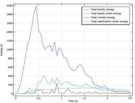
In the Settings window for Global, click Replace Expression in the upper-right corner of the y-Axis Data section. From the menu, choose Component 1 (comp1) > Solid Mechanics, Explicit Dynamics > Global > solid.Wk_tot - Total kinetic energy - J.
3
Click Add Expression in the upper-right corner of the y-Axis Data section. From the menu, choose Component 1 (comp1) > Solid Mechanics, Explicit Dynamics > Global > solid.Ws_tot - Total elastic strain energy - J.
4
Click Add Expression in the upper-right corner of the y-Axis Data section. From the menu, choose Component 1 (comp1) > Solid Mechanics, Explicit Dynamics > Global > solid.Wcnt_tot - Total contact energy - J.
5
Click Add Expression in the upper-right corner of the y-Axis Data section. From the menu, choose Component 1 (comp1) > Solid Mechanics, Explicit Dynamics > Global > solid.Wstb_tot - Total stabilization strain energy - J.
6
In the Total Energies toolbar, click  Plot.
Deformation
1
Click the  Zoom Extents button in the Graphics toolbar.
2
In the Model Builder window, under Results click Deformation.
3
In the Settings window for 3D Plot Group, locate the Data section.
4
From the Time (s) list, choose 1.
5
In the Deformation toolbar, click  Plot.
Appendix — Geometry Modeling Instructions
From the File menu, choose New.
New
In the New window, click  Model Wizard.
Model Wizard
1
In the Model Wizard window, click  3D.
2
Geometry 1
Block 1 (blk1)
1
In the Geometry toolbar, click  Block.
2
In the Settings window for Block, locate the Size and Shape section.
3
In the Width text field, type 1.25.
4
In the Depth text field, type 1.25.
5
In the Height text field, type 1.5.
6
Click to expand the Layers section. In the table, enter the following settings:
7
Find the Layer position subsection. Select the Left checkbox.
8
Select the Right checkbox.
9
Select the Front checkbox.
10
Select the Back checkbox.
Delete Entities 1 (del1)
1
In the Model Builder window, right-click Geometry 1 and choose Delete Entities.
2
On the object blk1, select Boundary 37 only.
Cylinder 1 (cyl1)
1
In the Geometry toolbar, click  Cylinder.
2
In the Settings window for Cylinder, locate the Size and Shape section.
3
In the Radius text field, type 0.15.
4
In the Height text field, type 1.25.
5
Locate the Position section. In the y text field, type 0.55.
6
In the z text field, type 0.85.
7
Locate the Axis section. From the Axis type list, choose x-axis.
Sphere 1 (sph1)
1
In the Geometry toolbar, click  Sphere.
2
In the Settings window for Sphere, locate the Size section.
3
In the Radius text field, type 0.15.
4
Locate the Position section. In the x text field, type 0.85.
5
In the y text field, type 0.75.
6
In the z text field, type 1.45.
7
Locate the Selections of Resulting Entities section. Find the Cumulative selection subsection. Click New.
8
In the New Cumulative Selection dialog, type Falling objects in the Name text field.
9
Sphere 2 (sph2)
1
In the Geometry toolbar, click  Sphere.
2
In the Settings window for Sphere, locate the Size section.
3
In the Radius text field, type 0.1.
4
Locate the Position section. In the x text field, type 0.2.
5
In the y text field, type 1.
6
In the z text field, type 1.45.
7
Locate the Selections of Resulting Entities section. Find the Cumulative selection subsection. From the Contribute to list, choose Falling objects.
Cylinder 2 (cyl2)
1
In the Geometry toolbar, click  Cylinder.
2
In the Settings window for Cylinder, locate the Size and Shape section.
3
In the Radius text field, type 0.06.
4
In the Height text field, type 0.6.
5
Locate the Position section. In the x text field, type 0.45.
6
In the y text field, type 0.25.
7
In the z text field, type 1.65.
8
Locate the Axis section. From the Axis type list, choose Cartesian.
9
In the x text field, type -0.2.
10
In the y text field, type 1.
11
In the z text field, type 0.
12
Locate the Selections of Resulting Entities section. Find the Cumulative selection subsection. From the Contribute to list, choose Falling objects.
Cylinder 3 (cyl3)
1
In the Geometry toolbar, click  Cylinder.
2
In the Settings window for Cylinder, locate the Size and Shape section.
3
In the Radius text field, type 0.07.
4
In the Height text field, type 0.6.
5
Locate the Position section. In the x text field, type 0.35.
6
In the y text field, type 0.95.
7
In the z text field, type 1.55.
8
Locate the Axis section. From the Axis type list, choose Cartesian.
9
In the x text field, type 1.
10
In the y text field, type 0.2.
11
In the z text field, type -0.2.
12
Locate the Selections of Resulting Entities section. Find the Cumulative selection subsection. From the Contribute to list, choose Falling objects.
Cylinder 4 (cyl4)
1
In the Geometry toolbar, click  Cylinder.
2
In the Settings window for Cylinder, locate the Size and Shape section.
3
In the Radius text field, type 0.2.
4
In the Height text field, type 0.1.
5
Locate the Position section. In the x text field, type 0.35.
6
In the y text field, type 0.35.
7
In the z text field, type 1.45.
8
Locate the Axis section. From the Axis type list, choose Cartesian.
9
In the x text field, type 0.1.
10
In the y text field, type 0.2.
11
Locate the Selections of Resulting Entities section. Find the Cumulative selection subsection. From the Contribute to list, choose Falling objects.
Cylinder 5 (cyl5)
1
In the Geometry toolbar, click  Cylinder.
2
In the Settings window for Cylinder, locate the Size and Shape section.
3
In the Radius text field, type 0.15.
4
In the Height text field, type 0.1.
5
Locate the Position section. In the x text field, type 0.65.
6
In the y text field, type 0.95.
7
In the z text field, type 1.25.
8
Locate the Axis section. From the Axis type list, choose Cartesian.
9
In the x text field, type 0.3.
10
In the y text field, type -0.1.
11
Locate the Selections of Resulting Entities section. Find the Cumulative selection subsection. From the Contribute to list, choose Falling objects.
Torus 1 (tor1)
1
In the Geometry toolbar, click  Torus.
2
In the Settings window for Torus, locate the Size and Shape section.
3
In the Major radius text field, type 0.15.
4
In the Minor radius text field, type 0.06.
5
Select the Interior faces checkbox.
6
Locate the Position section. In the x text field, type 0.55.
7
In the y text field, type 0.55.
8
In the z text field, type 1.25.
9
Locate the Axis section. From the Axis type list, choose Cartesian.
10
In the x text field, type 2.
11
In the y text field, type 1.
12
In the z text field, type -3.
13
Locate the Selections of Resulting Entities section. Find the Cumulative selection subsection. From the Contribute to list, choose Falling objects.
Torus 2 (tor2)
1
In the Geometry toolbar, click  Torus.
2
In the Settings window for Torus, locate the Size and Shape section.
3
In the Major radius text field, type 0.15.
4
In the Minor radius text field, type 0.07.
5
Select the Interior faces checkbox.
6
Locate the Position section. In the x text field, type 0.95.
7
In the y text field, type 0.3.
8
In the z text field, type 1.35.
9
Locate the Axis section. From the Axis type list, choose Cartesian.
10
In the x text field, type 1.
11
In the y text field, type 2.
12
In the z text field, type 3.
13
Locate the Selections of Resulting Entities section. Find the Cumulative selection subsection. From the Contribute to list, choose Falling objects.
Torus 3 (tor3)
1
In the Geometry toolbar, click  Torus.
2
In the Settings window for Torus, locate the Size and Shape section.
3
In the Major radius text field, type 0.2.
4
In the Minor radius text field, type 0.06.
5
In the Revolution angle text field, type 180.
6
Locate the Position section. In the x text field, type 0.35.
7
In the y text field, type 0.7.
8
In the z text field, type 1.25.
9
Locate the Axis section. From the Axis type list, choose Cartesian.
10
In the x text field, type 1.
11
In the y text field, type 3.
12
Locate the Selections of Resulting Entities section. Find the Cumulative selection subsection. From the Contribute to list, choose Falling objects.
Torus 4 (tor4)
1
In the Geometry toolbar, click  Torus.
2
In the Settings window for Torus, locate the Size and Shape section.
3
In the Major radius text field, type 0.22.
4
In the Minor radius text field, type 0.05.
5
In the Revolution angle text field, type 180.
6
Locate the Position section. In the x text field, type 0.9.
7
In the y text field, type 0.75.
8
In the z text field, type 1.05.
9
Locate the Axis section. From the Axis type list, choose Cartesian.
10
In the y text field, type -1.
11
In the z text field, type -2.
12
Locate the Selections of Resulting Entities section. Find the Cumulative selection subsection. From the Contribute to list, choose Falling objects.
Part Libraries
1
In the Geometry toolbar, click  Part Libraries.
2
In the Part Libraries window, select COMSOL Multiphysics > Platonic Solids > dodecahedron in the tree.
3
Click  Add to Geometry.
4
In the Select Part Variant dialog, select Specify circumradius in the Select part variant list.
5
Geometry 1
Dodecahedron 1 (pi1)
1
In the Model Builder window, under Component 1 (comp1) > Geometry 1 click Dodecahedron 1 (pi1).
2
In the Settings window for Part Instance, locate the Input Parameters section.
3
4
Locate the Position and Orientation of Output section. Find the Displacement subsection. In the xwi text field, type 1.
5
In the ywi text field, type 1.
6
In the zwi text field, type 1.25.
Dodecahedron 2 (pi2)
1
In the Geometry toolbar, click  Part Instance and choose Dodecahedron.
2
In the Settings window for Part Instance, locate the Input Parameters section.
3
4
Locate the Position and Orientation of Output section. Find the Displacement subsection. In the xwi text field, type 0.2.
5
In the ywi text field, type 0.2.
6
In the zwi text field, type 1.25.
Dodecahedron 3 (pi3)
1
In the Geometry toolbar, click  Part Instance and choose Dodecahedron.
2
In the Settings window for Part Instance, locate the Input Parameters section.
3
4
Locate the Position and Orientation of Output section. Find the Displacement subsection. In the xwi text field, type 0.6.
5
In the ywi text field, type 0.9.
6
In the zwi text field, type 0.95.
Explicit Selection 1 (sel1)
1
In the Geometry toolbar, click  Selections and choose Explicit Selection.
2
In the Settings window for Explicit Selection, locate the Entities to Select section.
3
From the Geometric entity level list, choose Object.
4
Select the objects pi1, pi2, and pi3 only.
5
Locate the Resulting Selection section. Find the Cumulative selection subsection. From the Contribute to list, choose Falling objects.
6
Clear the Keep selection checkbox.