|
|
|
|
•
|
|
1
|
|
2
|
|
3
|
Click Add.
|
|
4
|
Click
|
|
5
|
|
6
|
Click
|
|
1
|
|
2
|
|
1
|
|
2
|
|
3
|
|
4
|
|
5
|
|
1
|
|
2
|
|
3
|
|
4
|
|
5
|
|
1
|
|
2
|
|
3
|
|
1
|
|
2
|
|
3
|
|
4
|
|
5
|
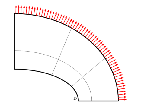
Select the object e3 only.
|
|
6
|
Click
|
|
1
|
|
2
|
|
3
|
|
4
|
|
5
|
|
6
|
|
1
|
|
2
|
|
3
|
|
4
|
|
5
|
|
6
|
|
1
|
In the Model Builder window, under Component 1 (comp1) right-click Materials and choose Blank Material.
|
|
2
|
|
1
|
|
2
|
|
3
|
From the list, choose Plane stress.
|
|
4
|
|
1
|
|
2
|
Select the Reduced integration checkbox.
|
|
3
|
|
1
|
|
1
|
|
3
|
|
4
|
|
5
|
|
1
|
|
2
|
|
3
|
|
5
|
Click
|
|
1
|
|
2
|
|
3
|
|
4
|
|
5
|
In the Show More Options dialog, in the tree, select the checkbox for the node Physics > Advanced Physics Options.
|
|
6
|
Click OK.
|
|
1
|
|
2
|
|
3
|
|
4
|
|
1
|
|
2
|
|
3
|
|
4
|
|
1
|
|
2
|
|
1
|
|
2
|
|
3
|
Click
|
|
1
|
|
2
|
|
3
|
Select the Modify model configuration for study step checkbox.
|
|
4
|
|
5
|
|
1
|
|
2
|
Go to the Add Study window.
|
|
3
|
|
4
|
Click the Add Study button in the window toolbar.
|
|
1
|
|
2
|
|
3
|
|
1
|
Go to the Add Study window.
|
|
2
|
|
3
|
Click the Add Study button in the window toolbar.
|
|
4
|
|
1
|
|
2
|
|
1
|
|
2
|
Select the Modify model configuration for study step checkbox.
|
|
3
|
|
4
|
|
1
|
|
2
|
Go to the Add Study window.
|
|
3
|
|
4
|
Click the Add Study button in the window toolbar.
|
|
1
|
|
2
|
Select the Modify model configuration for study step checkbox.
|
|
3
|
|
4
|
|
5
|
Clear the Modify model configuration for study step checkbox.
|
|
1
|
Go to the Add Study window.
|
|
2
|
|
3
|
Click the Add Study button in the window toolbar.
|
|
1
|
Go to the Add Study window.
|
|
2
|
|
3
|
Click the Add Study button in the window toolbar.
|
|
1
|
|
2
|
|
1
|
|
2
|
Select the Modify model configuration for study step checkbox.
|
|
3
|
|
4
|
|
1
|
Go to the Add Study window.
|
|
2
|
|
3
|
Click the Add Study button in the window toolbar.
|
|
1
|
|
2
|
|
3
|
|
1
|
|
2
|
Select the Modify model configuration for study step checkbox.
|
|
3
|
|
4
|
Right-click and choose Disable.
|
|
5
|
|
6
|
|
7
|
Click to expand the Mesh Selection section. In the table, enter the following settings:
|
|
1
|
Go to the Add Study window.
|
|
2
|
|
3
|
Click the Add Study button in the window toolbar.
|
|
1
|
|
2
|
|
3
|
|
1
|
|
2
|
Select the Modify model configuration for study step checkbox.
|
|
3
|
|
4
|
Right-click and choose Disable.
|
|
5
|
Locate the Mesh Selection section. In the table, enter the following settings:
|
|
1
|
Go to the Add Study window.
|
|
2
|
|
3
|
Click the Add Study button in the window toolbar.
|
|
4
|
|
1
|
|
2
|
|
3
|
|
1
|
|
2
|
Select the Modify model configuration for study step checkbox.
|
|
3
|
|
4
|
Right-click and choose Disable.
|
|
5
|
|
6
|
|
7
|
Locate the Mesh Selection section. In the table, enter the following settings:
|
|
1
|
|
2
|
|
3
|
Clear the Generate default plots checkbox.
|
|
4
|
|
1
|
|
2
|
|
3
|
Clear the Generate default plots checkbox.
|
|
4
|
|
1
|
|
2
|
|
3
|
Clear the Generate default plots checkbox.
|
|
4
|
|
1
|
|
2
|
|
3
|
Clear the Generate default plots checkbox.
|
|
4
|
|
1
|
|
2
|
|
3
|
Clear the Generate default plots checkbox.
|
|
4
|
|
1
|
|
2
|
|
3
|
Clear the Generate default plots checkbox.
|
|
4
|
|
1
|
|
2
|
|
3
|
Clear the Generate default plots checkbox.
|
|
4
|
|
1
|
|
2
|
|
3
|
Clear the Generate default plots checkbox.
|
|
4
|
|
1
|
|
2
|
|
3
|
Click
|
|
4
|
|
5
|
Click OK.
|
|
6
|
|
8
|
Click
|
|
1
|
|
2
|
|
1
|
|
3
|
|
4
|
|
5
|
|
6
|
|
7
|
|
8
|
Click to expand the Coloring and Style section. Find the Line markers subsection. From the Marker list, choose Asterisk.
|
|
9
|
|
10
|
|
1
|
|
2
|
|
3
|
|
4
|
Locate the Legends section. In the table, enter the following settings:
|
|
1
|
|
2
|
|
3
|
|
4
|
Locate the Legends section. In the table, enter the following settings:
|
|
1
|
|
2
|
|
3
|
|
4
|
Locate the Coloring and Style section. Find the Line style subsection. From the Line list, choose Dash-dot.
|
|
5
|
|
6
|
|
7
|
Locate the Legends section. In the table, enter the following settings:
|
|
1
|
|
2
|
|
3
|
|
4
|
|
5
|
Locate the Legends section. In the table, enter the following settings:
|
|
1
|
|
2
|
|
3
|
|
4
|
Locate the Legends section. In the table, enter the following settings:
|
|
1
|
|
2
|
|
3
|
|
4
|
Locate the Coloring and Style section. Find the Line style subsection. From the Line list, choose Dotted.
|
|
5
|
|
6
|
|
7
|
Locate the Legends section. In the table, enter the following settings:
|
|
1
|
|
2
|
|
3
|
|
4
|
|
5
|
Locate the Legends section. In the table, enter the following settings:
|
|
1
|
|
2
|
|
3
|
|
4
|
Locate the Legends section. In the table, enter the following settings:
|
|
1
|
|
2
|
|
3
|
|
4
|
|
5
|
|
6
|
|
7
|
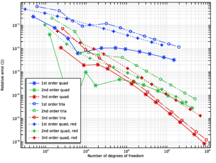
Select the y-axis log scale checkbox.
|
|
8
|
|
9
|
|
1
|
|
2
|
|
2
|
Go to the Find and Replace window.
|
|
3
|
|
4
|
|
5
|
|
6
|
|
7
|
Click OK.
|
|
8
|
Go to the Find and Replace window.
|
|
9
|
Click
|
|
10
|
|
1
|
|
2
|
|
1
|
|
2
|
|
2
|
Go to the Find and Replace window.
|
|
3
|
|
4
|
|
5
|
|
6
|
|
7
|
Click OK.
|
|
8
|
Go to the Find and Replace window.
|
|
9
|
Click
|
|
10
|
|
1
|
|
2
|
|
1
|
|
2
|
In the Settings window for 1D Plot Group, type Mesh Convergence sy at D (by DOFs) in the Label text field.
|
|
2
|
Go to the Find and Replace window.
|
|
3
|
|
4
|
|
5
|
|
6
|
|
7
|
Click OK.
|
|
8
|
Go to the Find and Replace window.
|
|
9
|
Click
|
|
10
|
|
1
|
In the Model Builder window, expand the Mesh Convergence sy at D (by DOFs) node, then click Results > Mesh Convergence sy at D (by DOFs).
|
|
2
|
|
3
|
|
4
|
|
1
|
|
2
|
|
3
|
Select the Transpose checkbox.
|
|
1
|
|
3
|
|
4
|
|
5
|
|
6
|
|
7
|
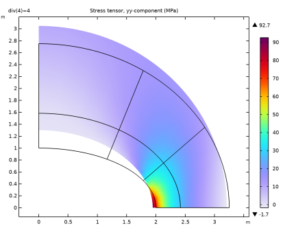
Click Replace Expression in the upper-right corner of the Expressions section. From the menu, choose Component 1 (comp1) > Solid Mechanics > Stress > Stress tensor (spatial frame) - N/m² > solid.sGpyy - Stress tensor, yy-component.
|
|
8
|
Locate the Expressions section. In the table, enter the following settings:
|
|
1
|
|
2
|
|
3
|
|
4
|
Locate the Expressions section. In the table, enter the following settings:
|
|
1
|
|
2
|
|
3
|
|
4
|
Locate the Expressions section. In the table, enter the following settings:
|
|
1
|
|
2
|
|
3
|
|
4
|
Locate the Expressions section. In the table, enter the following settings:
|
|
1
|
|
2
|
|
3
|
|
4
|
Locate the Expressions section. In the table, enter the following settings:
|
|
1
|
|
2
|
|
3
|
|
4
|
Locate the Expressions section. In the table, enter the following settings:
|
|
1
|
|
2
|
|
3
|
|
4
|
Locate the Expressions section. In the table, enter the following settings:
|
|
1
|
|
2
|
|
3
|
|
4
|
Locate the Expressions section. In the table, enter the following settings:
|
|
1
|
|
2
|
|
3
|
|
4
|
Locate the Expressions section. In the table, enter the following settings:
|
|
5
|
|
1
|
|
2
|
|
3
|
|
4
|
|
1
|
|
2
|
In the Settings window for Surface, click Replace Expression in the upper-right corner of the Expression section. From the menu, choose Component 1 (comp1) > Solid Mechanics > Stress > Stress tensor (spatial frame) - N/m² > solid.sGpyy - Stress tensor, yy-component.
|
|
3
|
|
1
|
|
2
|
|
3
|
Select the Show maximum and minimum values checkbox.
|
|
4
|