PDF

Elastic Cloaking with Polar Material
Introduction
An invisibility cloak aims at making inclusions neutral to probing incident wave fields. This can be achieved by surrounding the inclusion with a coating, which is designed so that outside of it the field produced by external sources remains exactly the same as that obtained in the case of free-field propagation. In that way, the cloak makes the inclusion impossible to be detected from measurements done outside of the cloak itself. In the context of linear elastodynamics, this implies that, in the most general case, the cloak should work for both P and S waves at the same time.
This example demonstrates how to implement the anisotropic linear elastic material model comprising non symmetric stresses, which is theoretically needed to obtain exact cloaking of an infinite cylinder when probed with the field generated by a point source (Ref. 1).
Model Definition
An infinite cylinder with radius r0 is covered by a cloak of radius r1. A unitary point load produces an oscillating force in the x direction at a circular frequency of 40 rad/s, producing a dipole excitation for P waves aligned with the x-axis, and at the same time a dipole excitation for S waves aligned with the y-axis. The geometrical parameters used in the model are listed in Table 1.
r0
r1
Governing Equations
The material properties required to obtain exact cloaking can be computed with the so-called transformation approach (Ref. 2). With this method, one starts by considering an unbounded domain occupied by a homogeneous isotropic linear elastic solid, where the displacement field u is governed by the elastodynamic Navier equations:
(1)
where a harmonic time dependence has been assumed. A mapping x' = χ(x) can be then introduced for points with radial coordinate r ≤ r1 as
(2)
This maps the origin onto a circle with radius r0 (the inner of the cloak) and points on a circle of radius r1 (the outer of the cloak) onto themselves. This means that the region of space inside the circle of radius r1 is radially compressed to fit into the annular region between r0 and r1. This map is applied then as a coordinate transformation to Equation 1, and the resulting equation can be shown to be equivalent to
(3)
where u' is used for
(4)
and
(5)
(6)
Here, F is the deformation gradient associated with the map χ, and J is its determinant, that is, the Jacobian of the transformation. Thus, the coefficients associated to the metric change induced by the change of coordinates are reinterpreted here as new material properties. If the annular region between r0 and r1 is filled with a linear elastic material whose properties are given by Equation 5 and Equation 6, then the solution outside the cloak will be exactly the same as the original free field propagation solution of Equation 1, while inside the cloak the displacement field will follow from Equation 4. Note that the same mapping χ equipped with a different definition of u' can lead to cloaks with different constitutive equations (Ref. 2). Here, the gauge transformation expressed by Equation 4 is chosen because it leads to a scalar density. Note, however, that the elasticity tensor defined in Equation 5 possesses the major symmetries
(7)
but not the minor ones
(8)
implying that the stress in the cloak is not symmetric.
Material Properties
The material properties of the cloak computed in cylindrical coordinates result in the eight non-null elastic moduli (plane strain) are listed in Table 2, along with the properties of the background isotropic hosting solid, whose elasticity tensor is specified through the two Lamé parameters λ and μ. Following Ref. 1, these are parameters that result in the same ratio between P- and S-wave speeds as that of fused silica.
(l+2μ)(r-r0)/r
(λ+2μ)r/(r-r0)
μ(r-r0)/r
μr/(r-r0)
ρcloak
ρ(r1/(r1-r0))2(r-r0)/r
The material properties of the cloak are implemented with the aid of the External Stress attribute under the Linear Elastic Material node. This allows to add a nonsymmetric stress component to the one computed via Hooke’s Law in the Linear Elastic Material. The total stress in the cloak is thus additively split into a part that can be obtained setting a standard symmetric elasticity tensor, plus a nonsymmetric stress that directly depends on the elements of the gradient of displacements.
This task is more easily performed when the equations are written in Cartesian coordinates. Equation 3 is thus firstly rewritten in component form in a Cartesian frame as
or, explicitly
Note indeed that the eight non-null moduli in cylindrical coordinates give rise in general to 16 non-null moduli in Cartesian coordinates. The four distinct elements of the stress tensor can be thus represented as
or equivalently as
where σsym can be written in Voigt notation as
and the external stress is
Results and Discussion
Figure 1 shows the displacement field for the free field case and the cloak case. It can be seen how the waves do not interact with the region inside the cloak, thus not producing scattering. At the same time, the cloaked region is protected from the probing incident radiation. Interference between P and S waves emitted from the point source can be observed.
Figure 1: The displacement magnitude in the free field scenario compared with the cloaked case.
Figure 2 shows the volumetric strain, highlighting the P wave part of the field. The point force applied in the horizontal direction produces a dipolar excitation for P waves aligned with the horizontal axis.
Figure 2: P wave emitted by the source in the free field and in the cloaked case scenario.
Figure 3 shows instead the S wave, via the local rotation expressed as the out-of-plane component of the curl of the displacement field. The point force in this case produces a dipolar excitation aligned with the vertical axis. Figure 2 together with Figure 3 clearly show how the cloak is capable of steering both P and S waves around the shielded area at the same time.
Figure 3: S wave emitted by the source in the free field and in the cloaked case scenario.
Notes About the COMSOL Implementation
The computational domain is truncated with a cylindrical Perfectly Matched Layer to represent propagation in an unbounded domain. A mapped mesh is used in the PML to make it work properly.
References
1. M. Brun, S. Guenneau, and A.B. Movchan, “Achieving control of in-plane elastic waves,” Appl. Phys. Lett., vol. 94, no. 6, p. 061903, 2009.
2. A.N. Norris, and A. Shuvalov, “Elastic cloaking theory,” Wave Motion, vol. 48, no. 6, pp. 525–538, 2011.
Application Library path: Structural_Mechanics_Module/Elastic_Waves/elastic_cloaking
Modeling Instructions
From the File menu, choose New.
New
In the New window, click  Model Wizard.
Model Wizard
1
In the Model Wizard window, click  2D.
2
In the Select Physics tree, select Structural Mechanics > Solid Mechanics (solid).
3
Click Add.
4
Click  Study.
5
In the Select Study tree, select General Studies > Frequency Domain.
6
Global Definitions
Geometrical Parameters
1
In the Model Builder window, under Global Definitions click Parameters 1.
2
In the Settings window for Parameters, type Geometrical Parameters in the Label text field.
3
Locate the Parameters section. In the table, enter the following settings:
Material Properties and Simulation Parameters
1
In the Home toolbar, click  Parameters and choose Add > Parameters.
2
In the Settings window for Parameters, type Material Properties and Simulation Parameters in the Label text field.
3
Locate the Parameters section. In the table, enter the following settings:
Geometry 1
Circle 1 (c1)
1
In the Geometry toolbar, click  Circle.
2
In the Settings window for Circle, locate the Size and Shape section.
3
In the Radius text field, type r2.
4
Click to expand the Layers section. In the table, enter the following settings:
5
Click  Build Selected.
Point 1 (pt1)
1
In the Geometry toolbar, click  Point.
2
In the Settings window for Point, locate the Point section.
3
In the x text field, type -((r2-Dpml-r1)/2+r1)*cos(pi/4).
4
In the y text field, type ((r2-Dpml-r1)/2+r1)*sin(pi/4).
5
Click  Build Selected.
Definitions
PML
1
In the Model Builder window, expand the Component 1 (comp1) > Definitions node.
2
Right-click Definitions and choose Selections > Explicit.
3
In the Settings window for Explicit, type PML in the Label text field.
4
Cloak
1
In the Definitions toolbar, click  Explicit.
2
In the Settings window for Explicit, type Cloak in the Label text field.
3
Background Solid
1
In the Definitions toolbar, click  Complement.
2
In the Settings window for Complement, type Background Solid in the Label text field.
3
Locate the Input Entities section. Under Selections to invert, click  Add.
4
In the Add dialog, in the Selections to invert list, choose PML and Cloak.
5
Background and Cloak
1
In the Definitions toolbar, click  Union.
2
In the Settings window for Union, type Background and Cloak in the Label text field.
3
Locate the Input Entities section. Under Selections to add, click  Add.
4
In the Add dialog, in the Selections to add list, choose Cloak and Background Solid.
5
Perfectly Matched Layer 1 (pml1)
1
In the Definitions toolbar, click  Perfectly Matched Layer.
2
In the Settings window for Perfectly Matched Layer, locate the Domain Selection section.
3
From the Selection list, choose PML.
4
Locate the Geometry section. From the Type list, choose Cylindrical.
First, set up the simulation for obtaining the free-field solution.
Solid Mechanics (solid)
Linear Elastic Material 1
1
In the Model Builder window, under Component 1 (comp1) > Solid Mechanics (solid) click Linear Elastic Material 1.
2
In the Settings window for Linear Elastic Material, locate the Linear Elastic Material section.
3
From the Specify list, choose Lamé parameters.
4
From the λ list, choose User defined. In the associated text field, type lambda.
5
From the μ list, choose User defined. In the associated text field, type mu.
6
From the ρ list, choose User defined. In the associated text field, type rho.
Point Load 1
1
In the Physics toolbar, click  Points and choose Point Load.
2
3
In the Settings window for Point Load, locate the Force section.
4
Specify the FP vector as
The mesh is set according to the requirements for the cloak scenario, where the material properties that tend to infinity need to be properly resolved.
Mesh 1
Mapped 1
1
In the Mesh toolbar, click  Mapped.
2
In the Settings window for Mapped, locate the Domain Selection section.
3
From the Geometric entity level list, choose Domain.
4
From the Selection list, choose PML.
Size
1
In the Model Builder window, click Size.
2
In the Settings window for Size, locate the Element Size section.
3
Click the Custom button.
4
Locate the Element Size Parameters section. In the Maximum element size text field, type wlengthS/12.
Distribution 1
1
In the Model Builder window, right-click Mapped 1 and choose Distribution.
2
3
In the Settings window for Distribution, locate the Distribution section.
4
In the Number of elements text field, type 7.
5
Click  Build Selected.
Mapped 2
1
In the Mesh toolbar, click  Mapped.
2
In the Settings window for Mapped, locate the Domain Selection section.
3
From the Geometric entity level list, choose Domain.
4
From the Selection list, choose Cloak.
Size 1
1
Right-click Mapped 2 and choose Size.
2
In the Settings window for Size, locate the Element Size section.
3
Click the Custom button.
4
Locate the Element Size Parameters section.
5
Select the Maximum element size checkbox. In the associated text field, type wlengthS/25.
Boundary Layers 1
1
In the Mesh toolbar, click  Boundary Layers.
2
In the Settings window for Boundary Layers, locate the Domain Selection section.
3
From the Geometric entity level list, choose Domain.
4
From the Selection list, choose Cloak.
Boundary Layer Properties
1
In the Model Builder window, click Boundary Layer Properties.
2
3
In the Settings window for Boundary Layer Properties, locate the Layers section.
4
From the Thickness specification list, choose All layers.
5
In the Number of layers text field, type 20.
6
Click  Build Selected.
Free Triangular 1
1
In the Mesh toolbar, click  Free Triangular.
2
In the Settings window for Free Triangular, click  Build All.
Free Field
1
In the Model Builder window, click Study 1.
2
In the Settings window for Study, type Free Field in the Label text field.
3
Locate the Study Settings section. Clear the Generate default plots checkbox.
Step 1: Frequency Domain
1
In the Model Builder window, under Free Field click Step 1: Frequency Domain.
2
In the Settings window for Frequency Domain, locate the Study Settings section.
3
In the Frequencies text field, type omega/2/pi.
4
In the Study toolbar, click  Compute.
Results
Displacement Field
1
In the Results toolbar, click  2D Plot Group.
2
In the Settings window for 2D Plot Group, type Displacement Field in the Label text field.
3
Click to expand the Title section. From the Title type list, choose Manual.
4
Clear the Parameter indicator text field.
5
In the Title text area, type Displacement magnitude (m).
6
Locate the Plot Settings section. Clear the Plot dataset edges checkbox.
Free Field
1
Right-click Displacement Field and choose Surface.
2
In the Settings window for Surface, type Free Field in the Label text field.
3
Locate the Coloring and Style section. From the Color table list, choose SpectrumLight.
4
In the Displacement Field toolbar, click  Plot.
Selection 1
1
Right-click Free Field and choose Selection.
2
In the Settings window for Selection, locate the Selection section.
3
From the Selection list, choose Background and Cloak.
Free Field
1
In the Model Builder window, click Free Field.
2
In the Settings window for Surface, click to expand the Range section.
3
Select the Manual color range checkbox.
4
In the Minimum text field, type 0.
5
In the Maximum text field, type 0.15.
6
In the Displacement Field toolbar, click  Plot.
7
In the Model Builder window, collapse the Free Field node.
P Wave
1
In the Results toolbar, click  2D Plot Group.
2
In the Settings window for 2D Plot Group, type P Wave in the Label text field.
3
Locate the Title section. From the Title type list, choose Manual.
4
Clear the Parameter indicator text field.
5
In the Title text area, type P wave (Volumetric strain).
6
Locate the Plot Settings section. Clear the Plot dataset edges checkbox.
Free Field
1
Right-click P Wave and choose Surface.
2
In the Settings window for Surface, type Free Field in the Label text field.
3
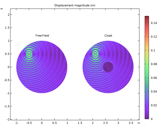
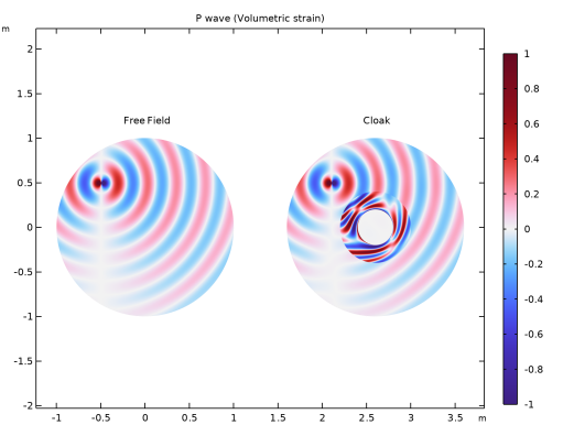
Click Replace Expression in the upper-right corner of the Expression section. From the menu, choose Component 1 (comp1) > Solid Mechanics > Strain > solid.evol - Volumetric strain - 1.
4
Locate the Coloring and Style section. From the Color table list, choose Wave.
Selection 1
1
Right-click Free Field and choose Selection.
2
In the Settings window for Selection, locate the Selection section.
3
From the Selection list, choose Background and Cloak.
Free Field
1
In the Model Builder window, click Free Field.
2
In the Settings window for Surface, locate the Range section.
3
Select the Manual color range checkbox.
4
In the Minimum text field, type -1.
5
In the Maximum text field, type 1.
6
In the P Wave toolbar, click  Plot.
7
In the Model Builder window, collapse the Free Field node.
S wave
1
In the Results toolbar, click  2D Plot Group.
2
In the Settings window for 2D Plot Group, type S wave in the Label text field.
3
Locate the Title section. From the Title type list, choose Manual.
4
Clear the Parameter indicator text field.
5
In the Title text area, type S wave (Curl of displacement, Z-component).
6
Locate the Plot Settings section. Clear the Plot dataset edges checkbox.
Surface 1
1
Right-click S wave and choose Surface.
2
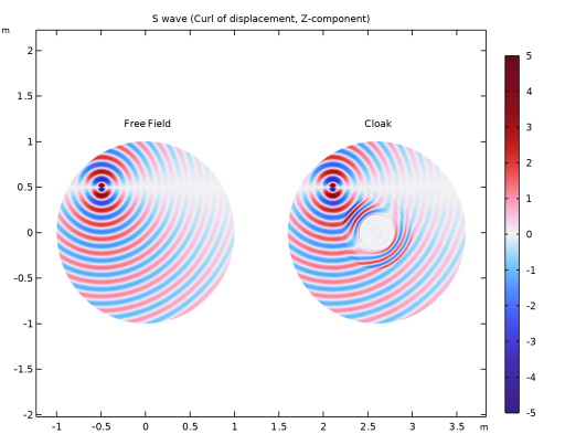
In the Settings window for Surface, click Replace Expression in the upper-right corner of the Expression section. From the menu, choose Component 1 (comp1) > Solid Mechanics > Displacement > Curl of displacement (material and geometry frames) > solid.curlUZ - Curl of displacement, Z-component.
3
Locate the Coloring and Style section. From the Color table list, choose Wave.
Selection 1
1
Right-click Surface 1 and choose Selection.
2
In the Settings window for Selection, locate the Selection section.
3
From the Selection list, choose Background and Cloak.
Surface 1
1
In the Model Builder window, click Surface 1.
2
In the Settings window for Surface, locate the Range section.
3
Select the Manual color range checkbox.
4
In the Minimum text field, type -5.
5
In the Maximum text field, type 5.
6
In the S wave toolbar, click  Plot.
7
In the Model Builder window, collapse the Surface 1 node.
Now, set up the simulation for the cloak. First, add a cylindrical coordinate system to define the radial dependence of the material properties.
Definitions
Cylindrical System 2 (sys2)
1
In the Definitions toolbar, click  Coordinate Systems and choose Cylindrical System.
2
In the Settings window for Cylindrical System, locate the Coordinate Names section.
3
From the Frame list, choose Material  (X, Y, Z).
Material Properties Cloak
1
In the Model Builder window, right-click Definitions and choose Variables.
The material properties of the cloak are defined in the cylindrical coordinate system. The elastic moduli are transformed to the global Cartesian coordinates. The computations have already been done, so you can directly import the final values.
2
In the Settings window for Variables, locate the Variables section.
3
Click  Load from File.
4
5
In the Label text field, type Material Properties Cloak.
Solid Mechanics (solid)
Linear Elastic Material Cloak
1
In the Physics toolbar, click  Domains and choose Linear Elastic Material.
2
In the Settings window for Linear Elastic Material, type Linear Elastic Material Cloak in the Label text field.
3
Locate the Domain Selection section. From the Selection list, choose Cloak.
4
Locate the Linear Elastic Material section. From the Material symmetry list, choose Anisotropic.
5
From the D list, choose User defined. Specify the associated matrix as
6
From the ρ list, choose User defined. In the associated text field, type rhocl.
External Stress 1
1
In the Physics toolbar, click  Attributes and choose External Stress.
2
In the Settings window for External Stress, locate the External Stress section.
3
From the Stress input list, choose Stress tensor (Nominal).
4
Specify the Pext matrix as
Add Study
1
In the Home toolbar, click  Add Study to open the Add Study window.
2
Go to the Add Study window.
3
Find the Studies subsection. In the Select Study tree, select General Studies > Frequency Domain.
4
Click the Add Study button in the window toolbar.
5
In the Home toolbar, click  Add Study to close the Add Study window.
Cloak
1
In the Settings window for Study, type Cloak in the Label text field.
2
Locate the Study Settings section. Clear the Generate default plots checkbox.
Step 1: Frequency Domain
1
In the Model Builder window, under Cloak click Step 1: Frequency Domain.
2
In the Settings window for Frequency Domain, locate the Study Settings section.
3
In the Frequencies text field, type omega/2/pi.
4
In the Study toolbar, click  Compute.
Results
Displacement Field
1
In the Model Builder window, under Results click Displacement Field.
2
In the Settings window for 2D Plot Group, click to expand the Plot Array section.
3
From the Array type list, choose Linear.
Cloak
1
In the Model Builder window, right-click Free Field and choose Duplicate.
2
In the Settings window for Surface, type Cloak in the Label text field.
3
Locate the Data section. From the Dataset list, choose Cloak/Solution 2 (sol2).
4
Click to expand the Title section. From the Title type list, choose None.
5
Click to expand the Inherit Style section. From the Plot list, choose Free Field.
6
In the Displacement Field toolbar, click  Plot.
7
Click the  Zoom Extents button in the Graphics toolbar.
Annotation Free Field
1
In the Model Builder window, right-click Displacement Field and choose Annotation.
2
In the Settings window for Annotation, type Annotation Free Field in the Label text field.
3
Locate the Annotation section. In the Text text field, type Free Field.
4
Locate the Position section. In the X text field, type 0.02.
5
In the Y text field, type 1.2.
6
Locate the Coloring and Style section. Clear the Show point checkbox.
7
From the Anchor point list, choose Center.
8
Click to expand the Plot Array section. Select the Manual indexing checkbox.
9
In the Displacement Field toolbar, click  Plot.
Annotation Cloak
1
Right-click Annotation Free Field and choose Duplicate.
2
In the Settings window for Annotation, type Annotation Cloak in the Label text field.
3
Locate the Annotation section. In the Text text field, type Cloak.
4
Locate the Plot Array section. In the Index text field, type 1.
5
In the Displacement Field toolbar, click  Plot.
P Wave
1
In the Model Builder window, under Results click P Wave.
2
In the Settings window for 2D Plot Group, locate the Plot Array section.
3
From the Array type list, choose Linear.
Cloak
1
In the Model Builder window, right-click Free Field and choose Duplicate.
2
In the Settings window for Surface, type Cloak in the Label text field.
3
Locate the Data section. From the Dataset list, choose Cloak/Solution 2 (sol2).
4
Locate the Title section. From the Title type list, choose None.
5
Locate the Inherit Style section. From the Plot list, choose Free Field.
6
In the P Wave toolbar, click  Plot.
7
Click the  Zoom Extents button in the Graphics toolbar.
Annotation Cloak, Annotation Free Field
1
In the Model Builder window, under Results > Displacement Field, Ctrl-click to select Annotation Free Field and Annotation Cloak.
2
P Wave
In the Model Builder window, under Results right-click P Wave and choose Paste Multiple Items.
Annotation Cloak, Annotation Free Field
In the P Wave toolbar, click  Plot.
S wave
1
In the Model Builder window, under Results click S wave.
2
In the Settings window for 2D Plot Group, locate the Plot Array section.
3
From the Array type list, choose Linear.
Free Field
1
In the Model Builder window, under Results > S wave click Surface 1.
2
In the Settings window for Surface, type Free Field in the Label text field.
Cloak
1
Right-click Free Field and choose Duplicate.
2
In the Settings window for Surface, type Cloak in the Label text field.
3
Locate the Data section. From the Dataset list, choose Cloak/Solution 2 (sol2).
4
Locate the Title section. From the Title type list, choose None.
5
Locate the Inherit Style section. From the Plot list, choose Free Field.
6
In the S wave toolbar, click  Plot.
Annotation Cloak, Annotation Free Field
1
In the Model Builder window, under Results > P Wave, Ctrl-click to select Annotation Free Field and Annotation Cloak.
2
S wave
In the Model Builder window, under Results right-click S wave and choose Paste Multiple Items.
Annotation Cloak, Annotation Free Field
In the S wave toolbar, click  Plot.
Modify the Free Field study to not include the cloak for future reruns.
Free Field
Step 1: Frequency Domain
1
In the Model Builder window, under Free Field click Step 1: Frequency Domain.
2
In the Settings window for Frequency Domain, locate the Physics and Variables Selection section.
3
Select the Modify model configuration for study step checkbox.
4
In the tree, select Component 1 (comp1) > Solid Mechanics (solid) > Linear Elastic Material Cloak.
5