|
|
|


|
1
|
|
2
|
|
3
|
Click Add.
|
|
4
|
Click
|
|
5
|
|
6
|
Click
|
|
1
|
|
2
|
|
3
|
Click
|
|
4
|
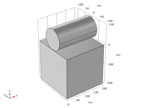
Browse to the model’s Application Libraries folder and double-click the file cylinder_roller_contact.txt.
|
|
1
|
|
2
|
|
1
|
|
2
|
|
3
|
|
1
|
|
2
|
|
3
|
|
4
|
|
5
|
|
6
|
|
7
|
Click
|
|
1
|
|
2
|
|
3
|
|
4
|
|
5
|
|
6
|
Click to expand the Layers section. In the table, enter the following settings:
|
|
7
|
Click
|
|
8
|
|
1
|
|
2
|
|
3
|
|
4
|
|
5
|
Click
|
|
1
|
|
2
|
|
3
|
|
4
|
|
1
|
|
2
|
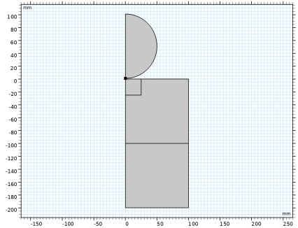
Select the object pt1 only.
|
|
3
|
|
4
|
|
5
|
|
6
|
Click
|
|
1
|
|
2
|
Click in the Graphics window and then press Ctrl+A to select all objects.
|
|
3
|
|
1
|
|
2
|
|
3
|
|
4
|
Clear the Create pairs checkbox.
|
|
1
|
|
2
|
On the object fin, select Domains 1–3 only.
|
|
3
|
|
1
|
|
3
|
|
4
|
Click to select the
|
|
1
|
|
2
|
|
3
|
|
1
|
|
1
|
|
1
|
|
3
|
|
4
|
|
1
|
|
3
|
|
4
|
|
1
|
In the Model Builder window, under Component 1 (comp1) right-click Materials and choose Blank Material.
|
|
2
|
|
1
|
|
3
|
|
1
|
In the Model Builder window, under Component 1 (comp1) > Solid Mechanics (solid) click Linear Elastic Material 1.
|
|
2
|
|
3
|
|
1
|
|
2
|
|
3
|
|
1
|
|
2
|
|
3
|
|
5
|
|
6
|
Locate the Element Size Parameters section.
|
|
7
|
|
8
|
Click
|
|
1
|
|
2
|
|
3
|
|
1
|
|
3
|
|
4
|
|
1
|
|
3
|
|
4
|
|
5
|
Click
|
|
1
|
|
2
|
|
3
|
Select the Auxiliary sweep checkbox.
|
|
4
|
Click
|
|
6
|
|
7
|
|
8
|
|
1
|
|
2
|
|
3
|
|
4
|
|
5
|
|
6
|
|
7
|
|
1
|
|
2
|
|
3
|
|
4
|
|
1
|
|
3
|
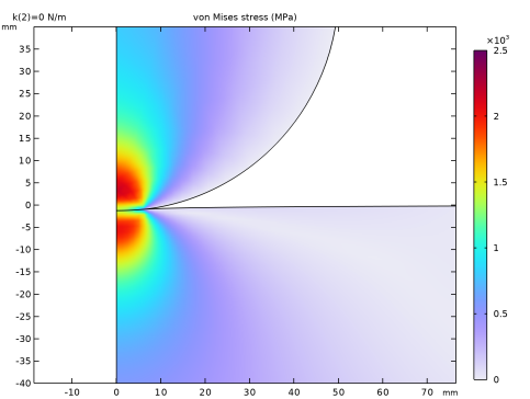
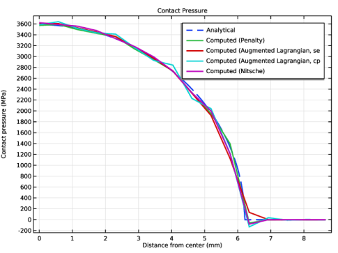
In the Settings window for Line Graph, click Replace Expression in the upper-right corner of the y-Axis Data section. From the menu, choose Component 1 (comp1) > Definitions > Variables > p_analytical - Analytical contact pressure - N/m².
|
|
4
|
|
5
|
Click Replace Expression in the upper-right corner of the x-Axis Data section. From the menu, choose Component 1 (comp1) > Geometry > Coordinate (spatial frame) > x - x-coordinate.
|
|
6
|
Click to expand the Coloring and Style section. Find the Line style subsection. From the Line list, choose Dashed.
|
|
7
|
|
8
|
|
9
|
|
11
|
|
1
|
|
2
|
|
3
|
|
4
|
Locate the Coloring and Style section. Find the Line style subsection. From the Line list, choose Solid.
|
|
5
|
Locate the Legends section. In the table, enter the following settings:
|
|
6
|
|
7
|
|
1
|
|
2
|
|
3
|
|
4
|
|
5
|
|
1
|
|
2
|
|
3
|
Click
|
|
4
|
|
5
|
Click OK.
|
|
6
|
|
7
|
From the list, choose Augmented Lagrangian.
|
|
1
|
|
2
|
|
3
|
|
1
|
|
2
|
Go to the Add Study window.
|
|
3
|
|
4
|
Right-click and choose Add Study.
|
|
5
|
|
1
|
|
2
|
Select the Modify model configuration for study step checkbox.
|
|
3
|
In the tree, select Component 1 (comp1) > Solid Mechanics (solid), Controls spatial frame > Contact 2.
|
|
4
|
Right-click and choose Disable.
|
|
5
|
|
6
|
Click
|
|
8
|
|
9
|
|
10
|
Clear the Generate default plots checkbox.
|
|
11
|
|
1
|
|
2
|
|
3
|
In the Model Builder window, expand the Study 2: Augmented Lagrangian, Segregated > Solver Configurations > Solution 2 (sol2) > Dependent Variables 1 node, then click Contact Pressure (comp1.solid.Tn_p1).
|
|
4
|
|
5
|
|
6
|
|
1
|
|
2
|
Go to the Add Study window.
|
|
3
|
|
4
|
Right-click and choose Add Study.
|
|
5
|
|
1
|
|
2
|
Select the Auxiliary sweep checkbox.
|
|
3
|
Click
|
|
5
|
|
6
|
|
7
|
Clear the Generate default plots checkbox.
|
|
8
|
|
1
|
|
2
|
|
3
|
In the Model Builder window, expand the Study 3: Augmented Lagrangian, Coupled > Solver Configurations > Solution 3 (sol3) > Dependent Variables 1 node, then click Contact Pressure (comp1.solid.Tn_p1).
|
|
4
|
|
5
|
|
6
|
|
1
|
In the Model Builder window, under Results > Contact Pressure right-click Line Graph 2 and choose Duplicate.
|
|
2
|
|
3
|
|
4
|
|
5
|
Locate the Legends section. In the table, enter the following settings:
|
|
1
|
|
2
|
|
3
|
|
4
|
Locate the Legends section. In the table, enter the following settings:
|
|
5
|
|
1
|
|
2
|
|
3
|
Click
|
|
4
|
|
5
|
Click OK.
|
|
6
|
|
7
|
From the list, choose Nitsche.
|
|
1
|
|
2
|
Go to the Add Study window.
|
|
3
|
|
4
|
Right-click and choose Add Study.
|
|
5
|
|
1
|
|
2
|
Select the Auxiliary sweep checkbox.
|
|
3
|
Click
|
|
5
|
|
6
|
|
7
|
Clear the Generate default plots checkbox.
|
|
8
|
|
1
|
|
2
|
Click
|
|
1
|
In the Model Builder window, under Results > Contact Pressure right-click Line Graph 4 and choose Duplicate.
|
|
2
|
|
3
|
|
4
|
|
5
|
Locate the Legends section. In the table, enter the following settings:
|
|
6
|
|
1
|
|
2
|
|
3
|
Select the Modify model configuration for study step checkbox.
|
|
4
|
In the tree, select Component 1 (comp1) > Solid Mechanics (solid), Controls spatial frame > Contact 1a.
|
|
5
|
Right-click and choose Disable.
|
|
6
|
In the tree, select Component 1 (comp1) > Solid Mechanics (solid), Controls spatial frame > Contact 2.
|
|
7
|
Right-click and choose Disable.
|
|
8
|
In the tree, select Component 1 (comp1) > Solid Mechanics (solid), Controls spatial frame > Contact 3.
|
|
9
|
Right-click and choose Disable.
|
|
1
|
In the Model Builder window, under Study 2: Augmented Lagrangian, Segregated click Step 1: Stationary.
|
|
2
|
|
3
|
In the tree, select Component 1 (comp1) > Solid Mechanics (solid), Controls spatial frame > Contact 3.
|
|
4
|
Right-click and choose Disable.
|
|
1
|
|
2
|
|
3
|
Select the Modify model configuration for study step checkbox.
|
|
4
|
In the tree, select Component 1 (comp1) > Solid Mechanics (solid), Controls spatial frame > Contact 3.
|
|
5
|
Right-click and choose Disable.
|