PDF

Torsion of an Isotropic Cosserat Elastic Cylinder
Introduction
The Cosserat theory of elasticity is one of the generalized continuum mechanics theories. It is also known as micropolar theory of elasticity, micropolar continuum mechanics or just micropolar elasticity. The theory incorporates, beside the displacement vector as in classical elasticity, the concept of the local rotation (or local spin) in the continuum, such that each point has six degrees of freedom: three translations and three rotations. The three rotations are also called microrotations. This theory can be used to model inhomogeneous materials, foams, masonries, bones, and so on.
This example demonstrates how to implement an isotropic linear Cosserat elasticity model through the use of the Weak Form PDE interface. A cylindrical bar made out of a Cosserat material is subject to a pure torsion where it is possible to observe the size effect on the response (Ref. 1).
Model Definition
A cylindrical bar with initial radius R0 and initial length L0 is axially twisted. It is fully constrained at one end and a prescribed rotation θ is applied on the opposite end. The parameter values are reported in Table 1.
R0
L0
θ
GOVERNING EQUATIONS
In Cosserat media each point has 6 degrees of freedom: three for the displacement vector u, and three microrotations (vector a). The constitutive equation for the Cauchy stress σ is augmented with an additional nonsymmetric term
(1)
This additional term depends on the difference of the skew-symmetric tensors W and A, and it can be seen as the force stress originated from the difference between the macrorotation and the local microrotation. These tensors are defined as follows:
(2)
(3)
where a1, a2, and a3 are the components of the microrotation vector a. The proportionality modulus μc, called Cosserat couple modulus (SI unit: Pa), relates the degree of coupling between the micro and macro rotations. The augmented stress is called force stress tensor, and it is used in the balance of linear momentum
(4)
In Cosserat theory, the conservation of angular momentum needs to be included as an additional equation, so that an additional tensor is necessary. It is called the couple stress or stress moment tensor, and it is defined as a linear combination of the gradient of the microrotation vector:
(5)
Here, α, β, and γ are the so-called first, second, and third microrotation parameters (SI unit: N). The couple stress tensor m will be symmetric, traceless, or nonsymmetric depending on their values. In Ref. 2 these parameters are written in terms of the Cosserat couple modulus μc and a length scale parameter. This example considers the following combination (the so-called pointwise positive case):
(6)
(7)
Here, Lc is the length scale that characterizes the Cosserat continuum. The couple stress tensor m is then nonsymmetric, and it can be written as follows:
(8)
The balance of angular momentum reads:
(9)
Here, the axial operator reads . The solution to the problem in terms of u and a is obtained by solving Equation 4 and Equation 9 together with the constitutive equations Equation 1 and Equation 8 and additional boundary conditions. In this example, only Dirichlet boundary conditions are considered.
WEAK FORM
Assuming no Neumann boundary condition are applied (no boundary loads), the weak contribution from the momentum conservation (Equation 4) is
(10)
The first term on the right-hand side is already included in the classical theory of elasticity and the second term is specific for Cosserat theory. The weak contribution coming from the angular momentum conservation (Equation 9) is
(11)
This contribution is not present in the classical theory of elasticity.
Material properties
An isotropic Cosserat medium needs six independent material parameters. Beside the Young’s modulus and Poisson’s ratio (E,ν), additional parameters include the three microrotation moduli (α, β, γ) and the couple modulus μc. Their values are reported in Table 2.
ν
μ
E/(2(1+ν))
α
β
γ
μLc2
μc
0.01μ, μ, 10μ
Boundary conditions
Dirichlet boundary conditions are applied in this example.
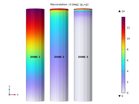
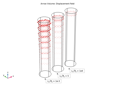
On the top surface, the displacement degrees of freedom u are constrained to reproduce a rigid rotation around the cylinder axis, whereas the microrotation degrees of freedom are free.
Results and Discussion
Figure 1 shows the size effect through the Cosserat length scale Lc on the reaction moment.
Figure 1: Torque versus scaled Cosserat length scale for different values of the Cosserat couple modulus μc as compared to the macroscopic shear modulus μ.
Figure 2 shows the reaction moment for the case with the smallest value of Cosserat couple module, μc = 0.01μ. Three different zones can be identified. The first zone, so-called linear Cauchy elasticity, extends up to Lc < 0.1R0. Here there is no size effect and the material behaves as a linear elastic solid (Zone I). There is a transition zone for values between 0.1R0 < Lc < 10R0, where the size effect on the solution (Zone II) is clearly visible. For higher values, 10R0 < Lc, the Cosserat effect dominates and the microrotation is nearly constant (Zone III).
Figure 2: Torque versus scaled Cosserat length scale. Three different zones can be identified.
The bar becomes stiffer as the ratio between the parameter Lc and the cylinder’s radius R0 increases. The bar twists only in the proximity of the constrained end (Figure 3) and the microrotation assume a constant value along the cylinder (Figure 4).
Figure 3: Macrorotation r3 for μc = μ and different values of the Cosserat length parameter Lc.
Figure 4: Microrotation, a3 for μc = μ and different values of the Cosserat length parameter Lc.
Figure 5: Displacement field before, during, and after transition.
Notes About the COMSOL Implementation
The equation for the balance of angular momentum is added through the use of a Weak Form PDE interface, where the three components of the microrotation vector are used as dependent variables.
The External Stress feature is used to account for the contribution of the asymmetric stress tensor that multiplies the macrorotation test function.An asymmetric stress can be entered using the Stress tensor (Nominal) option under Stress input. Alternatively, this contribution can be added directly in the Weak Form PDE interface together with the other additional terms.
A Rigid Connector is used to apply a rotation at the top of the cylindrical bar. Check the Evaluate reaction forces option to automatically compute the torque needed to twist the bar.
Default shape functions are used for the displacement field u. Linear Lagrange shape functions are used for the microrotation vector a.
A parametric study is used to loop over the Cosserat couple modulus and an auxiliary sweep to loop over the Cosserat length scale parameter.
A Fully Coupled solver is used to obtain convergence for higher values of the Cosserat couple modulus.
References
1. J. Jeong and H. Ramezani, “Implementation of the finite isotropic linear Cosserat models based on the weak form,” Proc. COMSOL Conf., Hannover, 2008.
2. J. Jeong and others, “A numerical study for linear isotropic Cosserat elasticity with conformally invariant curvature,” Z. Angew. Math. Mech. vol. 89, pp. 552–569, 2009.
Application Library path: Structural_Mechanics_Module/Material_Models/cosserat_torsion
Modeling Instructions
From the File menu, choose New.
New
In the New window, click  Model Wizard.
Model Wizard
1
In the Model Wizard window, click  3D.
2
In the Select Physics tree, select Structural Mechanics > Solid Mechanics (solid).
3
Click Add.
4
Click  Study.
5
In the Select Study tree, select General Studies > Stationary.
6
Global Definitions
General Parameters
1
In the Model Builder window, under Global Definitions click Parameters 1.
2
In the Settings window for Parameters, type General Parameters in the Label text field.
3
Locate the Parameters section. In the table, enter the following settings:
Cosserat Parameters
1
In the Home toolbar, click  Parameters and choose Add > Parameters.
Insert the parameters related to the Cosserat medium.
2
In the Settings window for Parameters, type Cosserat Parameters in the Label text field.
3
Locate the Parameters section. In the table, enter the following settings:
Geometry 1
1
In the Model Builder window, under Component 1 (comp1) click Geometry 1.
2
In the Settings window for Geometry, locate the Units section.
3
From the Length unit list, choose mm.
Cylinder 1 (cyl1)
1
In the Geometry toolbar, click  Cylinder.
2
In the Settings window for Cylinder, locate the Size and Shape section.
3
In the Radius text field, type R0.
4
In the Height text field, type L0.
5
Click  Build Selected.
Materials
Material 1 (mat1)
1
In the Model Builder window, under Component 1 (comp1) right-click Materials and choose Blank Material.
2
In the Settings window for Material, locate the Material Contents section.
3
Add Physics
1
In the Home toolbar, click  Add Physics to open the Add Physics window.
2
Go to the Add Physics window.
3
In the tree, select Mathematics > PDE Interfaces > Weak Form PDE (w).
4
Click to expand the Dependent Variables section. In the Field name (1) text field, type a.
5
In the Number of dependent variables text field, type 3.
6
In the Dependent variables (1) table, enter the following settings:
7
Click the Add to Component 1 button in the window toolbar.
8
In the Home toolbar, click  Add Physics to close the Add Physics window.
Microrotation Field
1
In the Settings window for Weak Form PDE, click to expand the Discretization section.
2
From the Element order list, choose Linear.
3
From the Frame list, choose Material.
4
In the Label text field, type Microrotation Field.
Define different tensors such as the microrotation tensor.
Definitions
Macrorotation Vector
1
In the Model Builder window, expand the Component 1 (comp1) > Definitions node.
2
Right-click Definitions and choose Variables.
3
In the Settings window for Variables, type Macrorotation Vector in the Label text field.
4
Locate the Variables section. In the table, enter the following settings:
5
Click the  Show More Options button in the Model Builder toolbar.
6
In the Show More Options dialog, in the tree, select the checkbox for the node General > Variable Utilities.
7
Macrorotation
1
In the Definitions toolbar, click  Variable Utilities and choose Matrix.
2
In the Settings window for Matrix, locate the Input Matrix section.
3
4
In the Label text field, type Macrorotation.
5
In the Name text field, type W.
Microrotation
1
In the Definitions toolbar, click  Variable Utilities and choose Matrix.
2
In the Settings window for Matrix, type Microrotation in the Label text field.
3
In the Name text field, type A.
4
Locate the Input Matrix section. In the table, enter the following settings:
Stress Moment Tensor
1
In the Definitions toolbar, click  Variable Utilities and choose Matrix.
2
In the Settings window for Matrix, locate the Input Matrix section.
3
4
In the Label text field, type Stress Moment Tensor.
5
In the Name text field, type M.
Asymmetric Stress Tensor
1
In the Definitions toolbar, click  Variable Utilities and choose Matrix.
2
In the Settings window for Matrix, type Asymmetric Stress Tensor in the Label text field.
3
In the Name text field, type Pc.
4
Locate the Input Matrix section. In the table, enter the following settings:
The symmetric Cauchy stress tensor is augmented with an asymmetric stress.
Solid Mechanics (solid)
Linear Elastic Material 1
In the Model Builder window, under Component 1 (comp1) > Solid Mechanics (solid) click Linear Elastic Material 1.
External Stress 1
1
In the Physics toolbar, click  Attributes and choose External Stress.
2
In the Settings window for External Stress, locate the External Stress section.
3
From the Stress input list, choose Stress tensor (Nominal).
4
Specify the Pext matrix as
Constrain one end of the bar and apply a rigid rotation at the other end.
Fixed Constraint 1
1
In the Physics toolbar, click  Boundaries and choose Fixed Constraint.
2
Rigid Connector 1
1
In the Physics toolbar, click  Boundaries and choose Rigid Connector.
2
3
In the Settings window for Rigid Connector, locate the Center of Rotation section.
4
From the list, choose Centroid of selected entities.
5
Locate the Prescribed Displacement at Center of Rotation section. Select the Prescribed in x direction checkbox.
6
Select the Prescribed in y direction checkbox.
7
Select the Prescribed in z direction checkbox.
8
Locate the Prescribed Rotation section. From the By list, choose Prescribed rotation.
9
Specify the Ω vector as
10
In the ϕ0 text field, type Theta0.
11
Click to expand the Reaction Force Settings section. Select the Evaluate reaction forces using weak constraints checkbox.
Center of Rotation: Boundary 1
1
In the Model Builder window, click Center of Rotation: Boundary 1.
2
The Cosserat medium introduces the microrotations as additional degrees of freedom. Their contribution to the weak form are now added.
Microrotation Field (w)
Weak Form PDE 1
1
In the Model Builder window, under Component 1 (comp1) > Microrotation Field (w) click Weak Form PDE 1.
2
In the Settings window for Weak Form PDE, locate the Weak Expressions section.
3
In the weak text-field array, type Pc11*test(A11)+Pc12*test(A12)+Pc13*test(A13)-M11*test(a1X)-M12*test(a1Y)-M13*test(a1Z) on the first row.
4
In the weak text-field array, type Pc21*test(A21)+Pc22*test(A22)+Pc23*test(A23)-M21*test(a2X)-M22*test(a2Y)-M23*test(a2Z) on the second row.
5
In the weak text-field array, type Pc31*test(A31)+Pc32*test(A32)+Pc33*test(A33)-M31*test(a3X)-M32*test(a3Y)-M33*test(a3Z) on the third row.
Dirichlet Boundary Condition 1
1
In the Physics toolbar, click  Boundaries and choose Dirichlet Boundary Condition.
2
Mesh 1
Free Quad 1
1
In the Mesh toolbar, click  More Generators and choose Free Quad.
2
Swept 1
In the Mesh toolbar, click  Swept.
Distribution 1
1
Right-click Swept 1 and choose Distribution.
2
In the Settings window for Distribution, locate the Distribution section.
3
In the Number of elements text field, type 30.
Size
1
In the Model Builder window, under Component 1 (comp1) > Mesh 1 click Size.
2
In the Settings window for Size, locate the Element Size section.
3
From the Predefined list, choose Finer.
4
Click  Build All.
Three Cosserat couple parameters are considered through the use of a parametric sweep. For each Cosserat couple parameter the Cosserat length scale is varied through an auxiliary sweep.
Study 1
1
In the Model Builder window, click Study 1.
2
In the Settings window for Study, locate the Study Settings section.
3
Clear the Generate default plots checkbox.
Step 1: Stationary
1
In the Model Builder window, under Study 1 click Step 1: Stationary.
2
In the Settings window for Stationary, click to expand the Study Extensions section.
3
Select the Auxiliary sweep checkbox.
4
5
Parametric Sweep
1
In the Study toolbar, click  Parametric Sweep.
2
In the Settings window for Parametric Sweep, locate the Study Settings section.
3
4
Solution 1 (sol1)
1
In the Study toolbar, click  Show Default Solver.
2
In the Model Builder window, expand the Solution 1 (sol1) node.
3
Right-click Study 1 > Solver Configurations > Solution 1 (sol1) > Stationary Solver 1 and choose Fully Coupled.
4
In the Study toolbar, click  Compute.
Results
Torque vs. Lc
1
In the Results toolbar, click  1D Plot Group.
2
In the Settings window for 1D Plot Group, type Torque vs. Lc in the Label text field.
3
Locate the Data section. From the Dataset list, choose Study 1/Parametric Solutions 1 (sol2).
4
Locate the Plot Settings section.
5
Select the x-axis label checkbox. In the associated text field, type L<sub>c</sub>/R<sub>0</sub>.
6
Select the y-axis label checkbox. In the associated text field, type Reaction moment z [N*m].
7
Locate the Axis section. Select the x-axis log scale checkbox.
8
Locate the Legend section. From the Position list, choose Upper left.
Global 1
1
Right-click Torque vs. Lc and choose Global.
2
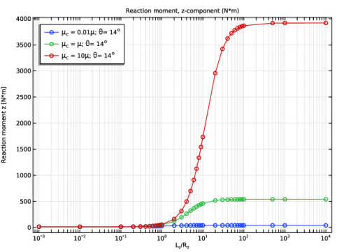
In the Settings window for Global, click Replace Expression in the upper-right corner of the y-Axis Data section. From the menu, choose Component 1 (comp1) > Solid Mechanics > Rigid connectors > Rigid Connector 1 > Reaction moment (spatial frame) - N·m > solid.rig1.RMz - Reaction moment, z-component.
3
Click to expand the Legends section. From the Legends list, choose Manual.
4
5
Click to expand the Coloring and Style section. Find the Line markers subsection. From the Marker list, choose Circle.
6
In the Torque vs. Lc toolbar, click  Plot.
Torque vs. Lc, muC = 0.01mu
1
In the Model Builder window, right-click Torque vs. Lc and choose Duplicate.
2
In the Settings window for 1D Plot Group, type Torque vs. Lc, muC = 0.01mu in the Label text field.
3
Locate the Data section. From the Parameter selection (muC) list, choose First.
4
In the Torque vs. Lc, muC = 0.01mu toolbar, click  Plot.
Point Graph 1
1
Right-click Torque vs. Lc, muC = 0.01mu and choose Point Graph.
2
3
In the Settings window for Point Graph, locate the y-Axis Data section.
4
In the Expression text field, type LcR0*0.003+13.
5
Locate the x-Axis Data section. From the Parameter list, choose Expression.
6
In the Expression text field, type 0.1.
7
Click to expand the Coloring and Style section. From the Color list, choose Black.
8
Click to expand the Title section. From the Title type list, choose None.
Point Graph 2
1
Right-click Point Graph 1 and choose Duplicate.
2
In the Settings window for Point Graph, locate the x-Axis Data section.
3
In the Expression text field, type 10.
4
In the Torque vs. Lc, muC = 0.01mu toolbar, click  Plot.
Torque vs. Lc, muC = 0.01mu
In the Torque vs. Lc, muC = 0.01mu toolbar, click  More Plots and choose Table Annotation.
Table Annotation 1
1
In the Settings window for Table Annotation, locate the Data section.
2
From the Source list, choose Local table.
3
4
Locate the Coloring and Style section. Clear the Show point checkbox.
5
Select the Show frame checkbox.
6
In the Torque vs. Lc, muC = 0.01mu toolbar, click  Plot.
Macrorotation, r3
1
In the Results toolbar, click  3D Plot Group.
2
In the Settings window for 3D Plot Group, type Macrorotation, r3 in the Label text field.
3
Locate the Data section. From the Dataset list, choose None.
4
Click to expand the Title section. From the Title type list, choose Manual.
5
In the Title text area, type Macrorotation: r3 [deg], (\mu<sub>C</sub>=\mu).
6
Clear the Parameter indicator text field.
7
Locate the Color Legend section. Select the Show maximum and minimum values checkbox.
Volume 1
1
Right-click Macrorotation, r3 and choose Volume.
2
In the Settings window for Volume, locate the Data section.
3
From the Dataset list, choose Study 1/Parametric Solutions 1 (sol2).
4
Locate the Expression section. In the Expression text field, type r3.
5
In the Unit field, type deg.
6
Locate the Coloring and Style section. From the Color table list, choose Prism.
Solution Array 1
1
Right-click Volume 1 and choose Solution Array.
2
In the Settings window for Solution Array, locate the Data section.
3
From the Parameter selection (muC) list, choose From list.
4
In the Parameter values (muC (Pa)) list box, select 3.8462E11.
5
From the Parameter selection (LcR0) list, choose From list.
6
In the Parameter values (LcR0) list, choose 0.001, 5, and 10000.
7
In the Macrorotation, r3 toolbar, click  Plot.
8
Click the  Go to XZ View button in the Graphics toolbar.
Annotation 1
1
In the Model Builder window, right-click Macrorotation, r3 and choose Annotation.
2
In the Settings window for Annotation, locate the Data section.
3
From the Dataset list, choose Study 1/Parametric Solutions 1 (sol2).
4
Locate the Position section. In the Z text field, type L0/2.
5
Locate the Annotation section. Select the LaTeX markup checkbox.
6
In the Text text field, type \textbf{ZONE 1}.
7
Locate the Coloring and Style section. Clear the Show point checkbox.
8
From the Anchor point list, choose Upper middle.
9
Click to expand the Plot Array section. Select the Manual indexing checkbox.
Annotation 2
1
Right-click Annotation 1 and choose Duplicate.
2
In the Settings window for Annotation, locate the Annotation section.
3
In the Text text field, type \textbf{ZONE 2}.
4
Locate the Plot Array section. In the Index text field, type 1.
Annotation 3
1
Right-click Annotation 2 and choose Duplicate.
2
In the Settings window for Annotation, locate the Annotation section.
3
In the Text text field, type \textbf{ZONE 3}.
4
Locate the Plot Array section. In the Index text field, type 2.
5
In the Macrorotation, r3 toolbar, click  Plot.
6
Click the  Show Grid button in the Graphics toolbar.
Microrotation, a3
1
In the Model Builder window, right-click Macrorotation, r3 and choose Duplicate.
2
In the Model Builder window, click Macrorotation, r3.1.
3
In the Settings window for 3D Plot Group, type Microrotation, a3 in the Label text field.
4
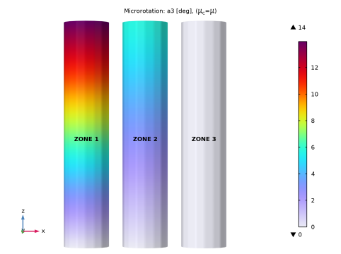
Locate the Title section. In the Title text area, type Microrotation: a3 [deg], (\mu<sub>C</sub>=\mu).
Volume 1
1
In the Model Builder window, click Volume 1.
2
In the Settings window for Volume, locate the Expression section.
3
In the Expression text field, type a3.
4
In the Microrotation, a3 toolbar, click  Plot.
5
Click the  Go to XZ View button in the Graphics toolbar.
6
Click the  Show Grid button in the Graphics toolbar.
Displacement, Arrow Plot
1
In the Results toolbar, click  3D Plot Group.
2
In the Settings window for 3D Plot Group, type Displacement, Arrow Plot in the Label text field.
3
Locate the Title section. From the Title type list, choose Custom.
4
Find the Solution subsection. Clear the Solution checkbox.
Arrow Volume 1
1
Right-click Displacement, Arrow Plot and choose Arrow Volume.
2
In the Settings window for Arrow Volume, locate the Data section.
3
From the Dataset list, choose Study 1/Parametric Solutions 1 (sol2).
4
Locate the Arrow Positioning section. Find the Z grid points subsection. In the Points text field, type 10.
5
Locate the Coloring and Style section.
6
Select the Scale factor checkbox. In the associated text field, type 3.
Solution Array 1
1
Right-click Arrow Volume 1 and choose Solution Array.
2
In the Settings window for Solution Array, locate the Data section.
3
From the Parameter selection (muC) list, choose From list.
4
In the Parameter values (muC (Pa)) list box, select 3.8462E11.
5
From the Parameter selection (LcR0) list, choose From list.
6
In the Parameter values (LcR0) list, choose 0.001, 5, and 10000.
7
In the Displacement, Arrow Plot toolbar, click  Plot.
Displacement, Arrow Plot
In the Model Builder window, under Results click Displacement, Arrow Plot.
Table Annotation 1
1
In the Displacement, Arrow Plot toolbar, click  More Plots and choose Table Annotation.
2
In the Settings window for Table Annotation, locate the Data section.
3
Select the LaTeX markup checkbox.
4
From the Source list, choose Local table.
5
6
Locate the Coloring and Style section. Select the Show frame checkbox.
7
In the Displacement, Arrow Plot toolbar, click  Plot.
8
Click the  Show Grid button in the Graphics toolbar.