
|
|
|

|
1
|
|
2
|
|
3
|
Click Add.
|
|
4
|
Click
|
|
5
|
|
6
|
Click
|
|
1
|
|
2
|
|
1
|
|
2
|
|
3
|
|
4
|
|
5
|
|
6
|
|
7
|
|
1
|
|
2
|
|
3
|
|
4
|
|
5
|
|
6
|
|
7
|
Locate the Layers section. In the table, enter the following settings:
|
|
8
|
Click
|
|
1
|
|
2
|
|
3
|
|
4
|
On the object c2, select Domain 1 only.
|
|
1
|
|
2
|
On the object c1, select Boundaries 2 and 3 only.
|
|
3
|
|
1
|
|
2
|
|
3
|
|
4
|
Click
|
|
1
|
|
2
|
|
3
|
|
5
|
Locate the Variables section. In the table, enter the following settings:
|
|
1
|
|
2
|
|
3
|
Click
|
|
4
|
|
5
|
Click OK.
|
|
6
|
|
7
|
Click to select the
|
|
8
|
Click
|
|
9
|
|
10
|
Click OK.
|
|
1
|
In the Model Builder window, under Component 1 (comp1) right-click Materials and choose Blank Material.
|
|
2
|
|
1
|
|
2
|
|
3
|
From the list, choose Augmented Lagrangian.
|
|
4
|
Locate the Contact Pressure Penalty Factor section. From the Penalty factor control list, choose Manual tuning.
|
|
5
|
|
1
|
|
2
|
|
3
|
|
4
|
|
5
|
In the Show More Options dialog, in the tree, select the checkbox for the node Physics > Advanced Physics Options.
|
|
6
|
Click OK.
|
|
7
|
|
8
|
Select the Store accumulated slip checkbox.
|
|
1
|
|
2
|
|
1
|
|
3
|
|
4
|
From the list, choose User defined.
|
|
5
|
|
6
|
|
7
|
|
1
|
|
2
|
|
3
|
Specify the F vector as
|
|
1
|
|
3
|
|
4
|
|
1
|
|
3
|
|
4
|
|
1
|
|
1
|
|
2
|
|
3
|
|
4
|
Click
|
|
1
|
|
2
|
|
3
|
Select the Plot checkbox.
|
|
4
|
|
5
|
|
6
|
Click
|
|
1
|
|
2
|
|
3
|
In the Model Builder window, expand the Study 1 > Solver Configurations > Solution 1 (sol1) > Dependent Variables 1 node, then click Contact Pressure (comp1.solid.Tn_p1).
|
|
4
|
|
5
|
|
6
|
In the Model Builder window, under Study 1 > Solver Configurations > Solution 1 (sol1) > Dependent Variables 1 click Friction Force (Spatial Frame) (comp1.solid.Tt_p1).
|
|
7
|
|
8
|
|
9
|
In the Model Builder window, expand the Study 1 > Solver Configurations > Solution 1 (sol1) > Stationary Solver 1 node, then click Parametric 1.
|
|
10
|
|
11
|
Select the Tuning of step size checkbox.
|
|
12
|
|
13
|
|
14
|
|
15
|
In the Model Builder window, expand the Study 1 > Solver Configurations > Solution 1 (sol1) > Stationary Solver 1 > Segregated 1 node, then click Solid Mechanics.
|
|
16
|
|
17
|
|
18
|
In the Model Builder window, under Study 1 > Solver Configurations > Solution 1 (sol1) right-click Compile Equations: Stationary and choose Run to Selected.
|
|
1
|
|
2
|
|
3
|
|
4
|
|
5
|
Locate the Coloring and Style section. Find the Line style subsection. From the Color list, choose Red.
|
|
6
|
|
7
|
|
8
|
|
9
|
|
10
|
|
1
|
|
2
|
|
3
|
|
4
|
|
5
|
|
1
|
|
2
|
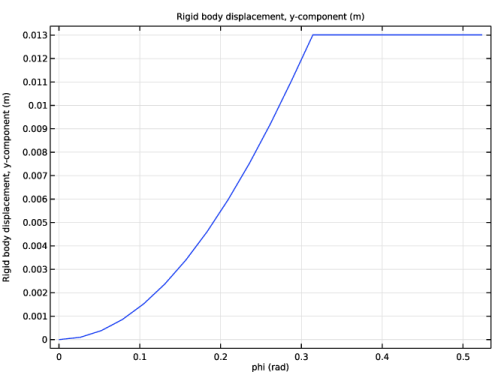
In the Settings window for Global, click Replace Expression in the upper-right corner of the y-Axis Data section. From the menu, choose Component 1 (comp1) > Solid Mechanics > Rigid connectors > Rigid Connector 1 > Rigid body displacement (spatial frame) - m > solid.rig1.v - Rigid body displacement, y-component.
|
|
3
|
|
1
|
|
2
|
|
3
|
|
4
|
|
5
|
|
6
|
Locate the Plot Settings section.
|
|
7
|
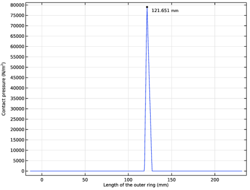
Select the y-axis label checkbox. In the associated text field, type Contact pressure (N/m<sup>2</sup>).
|
|
1
|
|
3
|
|
4
|
|
5
|
|
6
|
|
7
|
|
1
|
|
2
|
|
3
|
|
4
|
|
5
|
Clear the Show y-coordinate checkbox.
|
|
6
|
Select the Include unit checkbox.
|
|
7
|
|
1
|
|
1
|
|
2
|
|
3
|
|
4
|
|
1
|
|
2
|
|
3
|
|
1
|
|
2
|