
|
|
|
|
1
|
|
2
|
|
3
|
Click Add.
|
|
4
|
Click
|
|
5
|
|
6
|
Click
|
|
1
|
|
2
|
|
3
|
Click
|
|
4
|
Browse to the model’s Application Libraries folder and double-click the file cohesive_zone_debonding_parameters.txt.
|
|
1
|
|
2
|
|
3
|
|
1
|
|
2
|
|
3
|
|
4
|
|
5
|
|
6
|
Click to expand the Layers section. In the table, enter the following settings:
|
|
1
|
|
2
|
|
3
|
|
4
|
|
5
|
|
6
|
|
7
|
Locate the Layers section. In the table, enter the following settings:
|
|
8
|
|
1
|
In the Model Builder window, expand the Component 1 (comp1) > Definitions node, then click Boundary System 1 (sys1).
|
|
2
|
|
3
|
|
1
|
|
2
|
|
3
|
|
4
|
Browse to the model’s Application Libraries folder and double-click the file cohesive_zone_debonding_load_point_variables.txt.
|
|
1
|
|
2
|
|
3
|
|
5
|
|
1
|
|
2
|
|
3
|
|
5
|
|
1
|
|
2
|
Go to the Add Material window.
|
|
3
|
In the tree, select Composites > Laminae > Unidirectional fiber lamina: AS4/APC2 carbon/PEEK thermoplastic [fiber volume fraction 50%].
|
|
4
|
Right-click and choose Add to Global Materials.
|
|
5
|
|
1
|
|
2
|
|
1
|
|
3
|
|
4
|
|
5
|
|
1
|
|
2
|
|
3
|
|
4
|
|
1
|
|
2
|
|
3
|
|
4
|
|
5
|
|
6
|
|
7
|
|
8
|
|
9
|
|
10
|
In the Show More Options dialog, in the tree, select the checkbox for the node Physics > Equation Contributions.
|
|
11
|
Click OK.
|
|
1
|
|
1
|
|
1
|
|
2
|
|
4
|
|
5
|
|
1
|
|
2
|
|
4
|
|
5
|
|
1
|
|
3
|
|
4
|
|
1
|
|
3
|
|
4
|
|
1
|
|
2
|
|
4
|
|
5
|
|
6
|
|
7
|
Click OK.
|
|
8
|
|
9
|
Click
|
|
10
|
|
11
|
|
12
|
Click OK.
|
|
1
|
|
1
|
|
3
|
|
4
|
|
1
|
|
3
|
|
4
|
|
1
|
|
3
|
|
4
|
|
5
|
|
6
|
|
1
|
|
2
|
|
3
|
|
4
|
Click
|
|
1
|
|
2
|
|
3
|
Select the Include geometric nonlinearity checkbox.
|
|
4
|
|
5
|
|
6
|
|
7
|
Click
|
|
9
|
|
1
|
|
2
|
|
3
|
In the Model Builder window, expand the Study 1 > Solver Configurations > Solution 1 (sol1) > Dependent Variables 1 node, then click Global Equations 1 (comp1.ODE1).
|
|
4
|
|
5
|
|
6
|
|
7
|
In the Model Builder window, expand the Study 1 > Solver Configurations > Solution 1 (sol1) > Stationary Solver 1 node, then click Parametric 1.
|
|
8
|
|
9
|
Select the Tuning of step size checkbox.
|
|
10
|
|
11
|
|
12
|
In the Model Builder window, under Study 1 > Solver Configurations > Solution 1 (sol1) > Stationary Solver 1 click Fully Coupled 1.
|
|
13
|
|
14
|
|
15
|
|
1
|
|
2
|
|
3
|
|
4
|
|
1
|
|
2
|
|
3
|
Clear the Plot dataset edges checkbox.
|
|
4
|
|
5
|
|
1
|
|
2
|
|
1
|
|
2
|
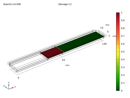
In the Settings window for Surface, click Replace Expression in the upper-right corner of the Expression section. From the menu, choose Component 1 (comp1) > Solid Mechanics > Contact > Adhesion > solid.bdmg - Damage - 1.
|
|
3
|
|
4
|
|
1
|
|
2
|
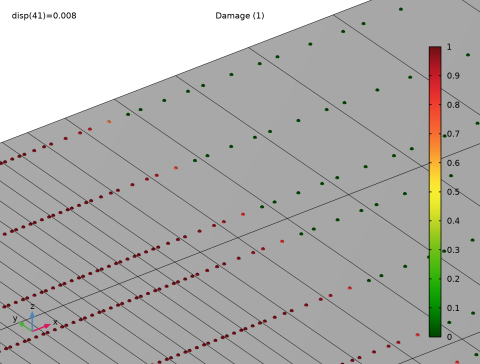
In the Settings window for 3D Plot Group, type Interface Health: Gauss Points in the Label text field.
|
|
1
|
|
2
|
|
3
|
|
4
|
|
5
|
|
6
|
|
7
|
|
8
|
|
9
|
|
10
|
|
1
|
|
2
|
|
3
|
Clear the Plot dataset edges checkbox.
|
|
1
|
|
2
|
|
3
|
|
1
|
|
1
|
|
2
|
|
3
|
|
4
|
|
1
|
|
2
|
|
3
|
|
4
|
|
1
|
|
2
|
|
4
|
|
5
|
|
6
|
|
7
|
|
1
|
|
2
|
|
1
|
|
2
|
|
4
|
|
5
|
 .
. .
.