PDF

Buckling Analysis of a Corrugated Conical Shell
Introduction
This tutorial model demonstrates how to perform a linear buckling analysis using cyclic symmetry with postprocessing on the full geometry. A conical shell with sixteen identical corrugations can be divided into sixteen sectors of symmetry. The model computes the critical load factor for the first buckling mode for the full shell geometry and compares it the value computed for a single sector with the cyclic symmetry boundary conditions applied on two sector boundaries. The results for one sector are in very good agreement with the computations on the full geometry, while the memory requirements are significantly reduced.
Model Definition
Figure 1 shows the shell geometry.
Figure 1: Full shell geometry.
The base radius is 3 cm, and the corrugation size is 1 mm. The structure height is 5 cm, and the shell thickness is 0.5 mm. The thickness is used as a modeling parameter in this tutorial to show its influence on the periodicity of the 1st buckling mode of the structure.
The geometry can be divided into sixteen identical parts, each represented by a sector with an angle θs = π/8 with respect to rotation around the z-axis; see Figure 2
Figure 2: Sector geometry.
The shell is made of aluminum. The bottom edge is fixed, and the load is applied vertically downward on the top edge.
Results and Discussion
Figure 3 shows the critical load factors computed using a unit sector for three different values and the shell thickness and different values of the azimuthal mode number. The latter parameter controls the periodicity with respect to the full geometry of the buckling mode computed using cyclic symmetry conditions. Thus, the angle of periodicity is ϕ = maθ, where the azimuthal mode number ma can vary from 0 to Ns/2, with Ns being the total number of sectors so that θs = 2π/Ns.
Figure 3: Critical load factor.
For example, Figure 4 shows the buckling mode computed using a unit sector for a shell thickness of 0.5 mm and azimuthal number ma = 4.
Figure 4: The first buckling mode with periodicity of four computed using a single sector and visualized on full geometry.
In Figure 3, the minimum value of the critical load factor computed for each given shell thickness indicates the symmetry type for the 1st buckling mode on the full geometry. Thus, Figure 5 show the 1st buckling mode computed on the full geometry for shell thickness of 0.5 mm.
Figure 5: The first buckling mode computed using full geometry.
Note that the modes computed using a unit sector (Figure 4) and the full geometry (Figure 4) differ only by a rigid body rotation around the z-axis; something that cannot be controlled during the full geometry buckling eigenvalue analysis. The computed critical load factors are in very good agreement with each other.
Notes About the COMSOL Implementation
To set up the cyclic symmetry conditions, you use the predefined functionality available in COMSOL Multiphysics within the Shell physics interface under the Periodic Condition boundary feature. This imposes the proper boundary coupling condition on the sector side boundaries. As the orientation of the edge normals needs to be specified, you add a cylindrical coordinate system to do that.
You visualize the results computed for one sector over the full geometry by making use of a predefined type of derived dataset called Sector 3D. Such a data set will be added automatically when the physics sets up cyclic symmetry using a Periodic Condition node.
Note that in general it is not possible to know the azimuthal mode number of the critical buckling load. Thus, you always have to perform a sweep to find the lowest value, as shown in this example.
The solution time for a sector is, however, much smaller than the solution time for the full geometry. So even though you have to solve the sector model several times using a parametric sweep, the total solution time will still be smaller than for the full model. The memory requirements when using the sector symmetry approach are much smaller than when using the full model.
Application Library path: Structural_Mechanics_Module/Buckling_and_Wrinkling/buckling_corrugated_shell
Modeling Instructions
From the File menu, choose New.
New
In the New window, click  Model Wizard.
Model Wizard
1
In the Model Wizard window, click  3D.
2
In the Select Physics tree, select Structural Mechanics > Shell (shell).
3
Click Add.
4
Click  Study.
5
In the Select Study tree, select Preset Studies for Selected Physics Interfaces > Linear Buckling.
6
Global Definitions
Parameters 1
1
In the Model Builder window, under Global Definitions click Parameters 1.
2
In the Settings window for Parameters, locate the Parameters section.
3
Create the sector geometry.
Geometry 1
Work Plane 1 (wp1)
In the Geometry toolbar, click  Work Plane.
Work Plane 1 (wp1) > Plane Geometry
In the Model Builder window, click Plane Geometry.
Work Plane 1 (wp1) > Parametric Curve 1 (pc1)
1
In the Work Plane toolbar, click  More Primitives and choose Parametric Curve.
2
In the Settings window for Parametric Curve, locate the Parameter section.
3
In the Maximum text field, type thetaS.
4
Locate the Expressions section. In the xw text field, type (Rc+hc*cos(Ns*s))*cos(s).
5
In the yw text field, type (Rc+hc*cos(Ns*s))*sin(s).
Extrude 1 (ext1)
1
In the Model Builder window, under Component 1 (comp1) > Geometry 1 right-click Work Plane 1 (wp1) and choose Extrude.
2
In the Settings window for Extrude, locate the Distances section.
3
4
Click to expand the Scales section. In the table, enter the following settings:
5
Locate the Selections of Resulting Entities section. Find the Cumulative selection subsection. Click New.
6
In the New Cumulative Selection dialog, type Sector in the Name text field.
7
8
In the Settings window for Extrude, click  Build Selected.
Also create the full geometry of the structure for verification computations.
Rotate 1 (rot1)
1
In the Geometry toolbar, click  Transforms and choose Rotate.
2
3
In the Settings window for Rotate, locate the Input section.
4
Select the Keep input objects checkbox.
5
Locate the Rotation section. In the Angle text field, type 360/Ns*range(1,1,Ns-1).
6
Locate the Selections on Input Objects section. Clear the Propagate selections to resulting objects checkbox.
7
Click  Build All Objects.
8
Click the  Zoom Extents button in the Graphics toolbar.
Add Material from Library
In the Home toolbar, click  Windows and choose Add Material from Library.
Add Material
1
Go to the Add Material window.
2
In the tree, select Built-in > Aluminum.
3
Right-click and choose Add to Component 1 (comp1).
Materials
Aluminum (mat1)
Click the  Go to XY View button in the Graphics toolbar.
Create a mapped mesh for the sector.
Mesh 1
Mapped 1
1
In the Mesh toolbar, click  More Generators and choose Mapped.
2
In the Settings window for Mapped, locate the Boundary Selection section.
3
From the Selection list, choose Sector.
Distribution 1
1
Right-click Mapped 1 and choose Distribution.
2
In the Settings window for Distribution, locate the Distribution section.
3
In the Number of elements text field, type 8.
4
Locate the Edge Selection section. From the Selection list, choose Sector.
5
Locate the Distribution section. Select the Equidistant checkbox.
6
Click  Build All.
Add a cylindrical coordinate system which you will use in the periodic boundary conditions to specify the edge orientation.
Definitions
Cylindrical System 2 (sys2)
1
In the Definitions toolbar, click  Coordinate Systems and choose Cylindrical System.
2
In the Settings window for Cylindrical System, locate the Coordinate Names section.
3
From the Frame list, choose Material  (X, Y, Z).
Set up the physics on the sector.
Shell (shell)
1
In the Model Builder window, under Component 1 (comp1) click Shell (shell).
2
In the Settings window for Shell, locate the Boundary Selection section.
3
From the Selection list, choose Sector.
Thickness and Offset 1
1
In the Model Builder window, under Component 1 (comp1) > Shell (shell) click Thickness and Offset 1.
2
In the Settings window for Thickness and Offset, locate the Thickness and Offset section.
3
In the d0 text field, type th.
Fixed Constraint 1
1
In the Physics toolbar, click  Edges and choose Fixed Constraint.
Select the bottom edge of the sector to be fixed.
2
Edge Load 1
1
In the Physics toolbar, click  Edges and choose Edge Load.
Specify the buckling load.
Select the top edge of the sector.
2
3
In the Settings window for Edge Load, locate the Force section.
4
From the Load type list, choose Force per reference area.
5
Specify the fA vector as
It is conventional to use a unit load, but the load value is in fact arbitrary. The actual buckling load will be a product of this value and the critical load factor computed during the buckling study.
Periodic Condition 1
1
In the Physics toolbar, click  Edges and choose Periodic Condition.
Select the side edges of the sector.
2
3
Right-click Periodic Condition 1 and choose Manual Destination Selection.
4
In the Settings window for Periodic Condition, locate the Destination Selection section.
5
6
Click  Clear Selection.
7
Click  Paste Selection.
8
In the Paste Selection dialog, type 43 in the Selection text field.
9
It is conventional to use a unit load, but the load value is in fact arbitrary. The actual buckling load will be a product of this value and the critical load factor computed during the buckling study.
10
In the Settings window for Periodic Condition, locate the Periodicity Settings section.
11
From the Type of periodicity list, choose Cyclic symmetry.
12
In the θS text field, type thetaS.
13
In the m text field, type ma.
Use the cylindrical coordinate system to specify the orientation of the source and destination edges.
14
Click to expand the Orientation of Source section. From the Transform to intermediate map list, choose Cylindrical System 2 (sys2).
15
Click to expand the Orientation of Destination section. From the Transform to intermediate map list, choose Cylindrical System 2 (sys2).
Set up a parametric sweep to find the first buckling modes for shell of various thickness.
Study 1: Sector
1
In the Model Builder window, click Study 1.
2
In the Settings window for Study, type Study 1: Sector in the Label text field.
Parametric Sweep
1
In the Study toolbar, click  Parametric Sweep.
2
In the Settings window for Parametric Sweep, locate the Study Settings section.
3
4
Step 2: Linear Buckling
1
In the Model Builder window, click Step 2: Linear Buckling.
2
In the Settings window for Linear Buckling, click to expand the Study Extensions section.
3
Select the Auxiliary sweep checkbox.
4
5
6
In the Study toolbar, click  Compute.
Plot all computed buckling critical load factors.
Results
Critical load factor
1
In the Results toolbar, click  1D Plot Group.
2
In the Settings window for 1D Plot Group, type Critical load factor in the Label text field.
3
Click to expand the Title section. From the Title type list, choose Manual.
4
In the Title text area, type Critical load factor.
5
Locate the Axis section. Select the y-axis log scale checkbox.
6
Locate the Grid section. Select the Manual spacing checkbox.
7
Locate the Axis section. Select the Manual axis limits checkbox.
8
In the x minimum text field, type -0.1.
9
In the x maximum text field, type 8.1.
10
In the y minimum text field, type 1E7.
11
In the y maximum text field, type 1E9.
12
Locate the Legend section. From the Position list, choose Lower left.
Global 1
1
Right-click Critical load factor and choose Global.
2
In the Settings window for Global, locate the Data section.
3
From the Dataset list, choose Study 1: Sector/Parametric Solutions 1 (sol3).
4
From the Parameter selection (th) list, choose From list.
5
In the Parameter values (th (mm)) list box, select 0.1.
6
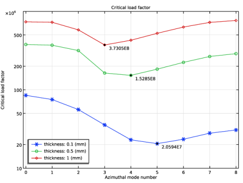
Click Replace Expression in the upper-right corner of the y-Axis Data section. From the menu, choose Component 1 (comp1) > Shell > shell.LFcrit - Critical load factor.
7
Locate the x-Axis Data section. From the Axis source data list, choose Inner solutions.
8
From the Parameter list, choose Expression.
9
In the Expression text field, type ma.
10
Click to expand the Coloring and Style section. Find the Line markers subsection. From the Marker list, choose Cycle.
11
Click to expand the Legends section. Find the Include subsection. Clear the Solution checkbox.
12
Clear the Description checkbox.
13
Find the Prefix and suffix subsection. In the Suffix text field, type thickness: eval(th, mm) (mm).
14
In the Critical load factor toolbar, click  Plot.
Graph Marker 1
1
Right-click Global 1 and choose Graph Marker.
2
In the Settings window for Graph Marker, locate the Display section.
3
From the Display list, choose Min.
4
Locate the Text Format section. In the Precision text field, type 5.
Global 2
1
In the Model Builder window, under Results > Critical load factor right-click Global 1 and choose Duplicate.
2
In the Settings window for Global, locate the Data section.
3
In the Parameter values (th (mm)) list box, select 0.5.
Global 3
1
Right-click Global 2 and choose Duplicate.
2
In the Settings window for Global, locate the Data section.
3
In the Parameter values (th (mm)) list box, select 1.
4
In the Critical load factor toolbar, click  Plot.
The software automatically generates a special sector data set to visualize the periodic solution for a full geometry. Inspect the case, for which the shell thickness is 0.5 mm, and azimuthal mode number is four.
Mode Shape, Full Geometry (shell)
1
In the Model Builder window, under Results click Mode Shape, Full Geometry (shell).
2
In the Settings window for 3D Plot Group, locate the Data section.
3
From the Parameter value (th (mm)) list, choose 0.5.
4
From the Parameter value (ma) list, choose 4.
5
Locate the Plot Settings section. Clear the Plot dataset edges checkbox.
6
In the Mode Shape, Full Geometry (shell) toolbar, click  Plot.
You use this case to compare the result with that computed using the true full geometry for the same shell thickness.
Add one more Shell physics interface, a new mesh, and a new buckling study to compute using the full geometry.
Add Physics
1
In the Home toolbar, click  Windows and choose Add Physics.
2
Go to the Add Physics window.
3
In the tree, select Structural Mechanics > Shell (shell).
4
Click the Add to Component 1 button in the window toolbar.
Shell 2 (shell2)
Thickness and Offset 1
1
In the Settings window for Thickness and Offset, locate the Thickness and Offset section.
2
In the d0 text field, type th.
Fixed Constraint 1
1
In the Physics toolbar, click  Edges and choose Fixed Constraint.
Select all bottom edges to be fixed.
2
Specify the buckling load.
Edge Load 1
1
In the Physics toolbar, click  Edges and choose Edge Load.
Select all top edges.
2
3
In the Settings window for Edge Load, locate the Force section.
4
From the Load type list, choose Force per reference area.
5
Specify the fA vector as
Mesh 2
In the Mesh toolbar, click Add Mesh and choose Add Mesh.
Reference 1
1
In the Mesh toolbar, click  Modify and choose Reference.
2
In the Settings window for Reference, locate the Reference section.
3
From the Mesh list, choose Mesh 1.
Copy Face 1
1
In the Mesh toolbar, click  Copy and choose Copy Face.
2
In the Settings window for Copy Face, locate the Source Boundaries section.
3
From the Selection list, choose Sector.
4
Locate the Destination Boundaries section. Click to select the  Activate Selection toggle button.
Select all other boundaries as destination.
5
Click  Paste Selection.
6
In the Paste Selection dialog, type 1-15 in the Selection text field.
7
8
In the Settings window for Copy Face, click  Build All.
Add a new study to compute using the full geometry.
Add Study
1
In the Home toolbar, click  Windows and choose Add Study.
2
Go to the Add Study window.
3
Find the Studies subsection. In the Select Study tree, select Preset Studies for Selected Physics Interfaces > Linear Buckling.
4
Study 2
Step 1: Stationary
1
In the Model Builder window, under Study 2 click Step 1: Stationary.
2
In the Settings window for Stationary, locate the Physics and Variables Selection section.
3
Select the Modify model configuration for study step checkbox.
4
In the tree, select Component 1 (comp1) > Shell (shell).
5
Right-click and choose Disable in Model.
Step 2: Linear Buckling
1
In the Model Builder window, click Step 2: Linear Buckling.
2
In the Settings window for Linear Buckling, locate the Physics and Variables Selection section.
3
Select the Modify model configuration for study step checkbox.
4
In the tree, select Component 1 (comp1) > Shell (shell).
5
Right-click and choose Disable in Model.
6
In the Model Builder window, click Study 2.
7
In the Settings window for Study, type Study 2: Verification in the Label text field.
8
In the Study toolbar, click  Compute.
Results
Mode Shape, Verification (shell2)
1
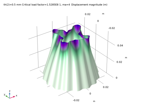
In the Settings window for 3D Plot Group, type Mode Shape, Verification (shell2) in the Label text field.
2
Locate the Plot Settings section. Clear the Plot dataset edges checkbox.
3
In the Mode Shape, Verification (shell2) toolbar, click  Plot.
4
Click the  Go to Default View button in the Graphics toolbar.
Compare the result to that computed using a single sector.