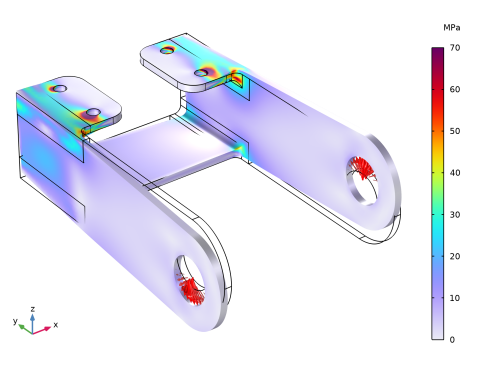
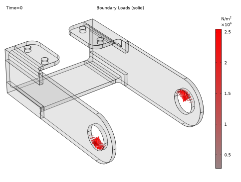
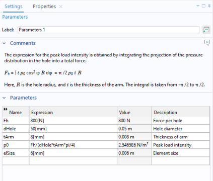
PDF

Bracket — Static Analysis
Introduction
The various examples based on a bracket geometry form a suite of tutorials which summarizes the fundamentals when modeling structural mechanics problems in COMSOL Multiphysics and the Structural Mechanics Module.
This is the first model in the suite, showing a linear static analysis. It includes the definition of material properties and boundary conditions. After the solution is computed, you learn how to analyze the results.
Model Definition
The model used in this guide is a bracket made of steel. This type of bracket can be used to install an actuator that is mounted on a pin placed between the two holes in the bracket arms. The geometry is shown in Figure 1.
Figure 1: Bracket geometry.
In this analysis, the mounting bolts are assumed to be fixed and securely bonded to the bracket. One of the arms is loaded upward and the other downward. The loads are applied as a pressure on the inner surfaces of the holes, and their intensity is p = p0 cos(α), where α is the angle from the direction of the load resultants. This is a common assumption for pins with a small clearance. Figure 2 below shows the loads applied to the bracket.
Figure 2: Load distribution in the bracket arms.
The resultant load in each hole is Fh = 800 N. The pressure intensity p0 can be determined from an integration of the projected pressure
(1)
where t is the thickness of the arm, and d is the diameter of the hole.
Results
Figure 3 shows the von Mises stress distribution together with an exaggerated (automatically scaled) picture of the deformation. The high stress values are located in the vicinity of the mounting bolts and at the transition between the plates. The stress at the bolt holes is, to some extent, an effect of the assumed boundary condition which causes a singularity. This is a common situation in structural mechanics models.
The von Mises equivalent stress is a good measure of the safety against plastic deformations for a material like steel which essentially is independent to the sign and orientation of the stresses.
Figure 3: Von Mises stress distribution in the bracket under a twisting load.
In Figure 4, you can see that the bracket base remains fixed while only the arms are deformed. The maximum total displacement is about 0.25 mm, which is in agreement with the assumption of small deformations.
Figure 4: Total displacement.
Figure 5 shows the principal stresses in the bracket. The largest principal stress is shown with red arrows, the intermediate principal stress with green arrows, and the smallest principal stress with blue arrows. Since a state of plane stress prevails in large parts of the structure (the thin plates) one of the principal stresses is mostly zero. Note that the principal stress arrows in this figure are shown using a logarithmic scale. This will give a good overview of the orientation of the stress components. With a linear scale, only a few arrows at the stress concentrations would be visible.
Figure 5: Principal stress in the bracket left arm (logarithmic scale).
In Figure 6 and Figure 7, you can see the stress variation along an edge of the fillet connecting one of the arms of the bracket to the mounting plate. The difference between these two plots is that in the second one, there is no averaging between adjacent elements. By disabling averaging in graphs or color plots, you can get an indication of the discretization error in the solution. The default stress plot (Figure 3) actually has a setting making the averaging optional. If the stress jump between two adjacent elements is larger than a certain threshold value, no averaging is performed.
Figure 6: First principal stress along the fillet with the highest stress.
Figure 7: First principal stress along the fillet with the highest stress. No averaging between adjacent elements.
If the bracket would have been made from cast iron, rather than steel, the von Mises stress as shown in Figure 3 is a less suitable criterion, since cast iron is more sensitive to tension than compression. In COMSOL, you can find many failure criteria, suitable for materials with more sophisticated failure modes.
For a cast iron, it is possible to use the Rankine criterion. In this case, the largest principal stress in each point is checked against the allowed tensile stress, while the smallest principal stress is checked against the allowed compressive stress. Here it is assumed that the allowed values are
In Figure 8, the failure index for the Rankine criterion is shown. Values above 1 indicate failure. This happens around the bolt holes, there the stresses are unrealistic anyway.
Figure 8: Failure in using a Rankine criterion.
It can be noted that with the Rankine criterion, the risk of failure is no longer symmetric between the right and left sides of the bracket.
Notes About the COMSOL Implementation
In this model, the possibility to add comments to nodes in the Model Builder is utilized. This can be useful when some expressions in the settings are not obvious to someone else using your model, or even when you yourself revisit it later. An example is shown in Figure 9.
Figure 9: The Settings tab for the Parameters node with an explanatory comment added.
You add and modify comments in the Properties tab for a certain node. This tab is not shown by default. To open the Properties tab, right-click on the current node, and select Properties and Comments. You can now enter a text, and there are also a number of formatting tools as shown in Figure 10. Once you have added a comment for a node in the model, this comment will be visible in the Settings tab.
Figure 10: The Properties tab for the Parameters node, where the comment text is maintained.
Note that the complex expressions in Figure 10 is not the way you typically enter comments. It is an effect of applying formatting tools from the toolbars.
Application Library path: Structural_Mechanics_Module/Tutorials/bracket_static
Modeling Instructions
This example is the same as described in the Introduction to the Structural Mechanics Module document. If you are new to COMSOL Multiphysics, that may be a better starting point, since it contains a more detailed description.
Note that part of the instructions below are not essential for performing the analysis. Rather, they are intended to showcase some useful tools. Examples of such instructions are the assignments of colors to geometrical parts, as well as many adjustments to the plots.
The first step to build a model is to open COMSOL and then specify the type of analysis you want to do - in this case, a stationary, solid mechanics analysis.
From the File menu, choose New.
New
In the New window, click  Model Wizard.
Model Wizard
1
In the Model Wizard window, click  3D.
2
In the Select Physics tree, select Structural Mechanics > Solid Mechanics (solid).
3
Click Add.
4
Click  Study.
5
In the Select Study tree, select General Studies > Stationary.
6
Global Definitions
It is good modeling practice to gather constants and parameters in one place so that you can change them easily. Using parameters will also improve the readability of your input data.
Parameters 1
1
In the Model Builder window, under Global Definitions click Parameters 1.
2
In the Settings window for Parameters, locate the Parameters section.
3
In any node in the Model Builder, you can add comments to explain the settings. In this example, you may want to explain the expression for the peak load intensity. How to do that is shown in Figure 9 and Figure 10.
Geometry 1
The next step is to create your geometry, which also can be imported from an external program. COMSOL Multiphysics supports a multitude of CAD programs and file formats. In this example, import a file in the COMSOL Multiphysics geometry file format (.mphbin).
Import 1 (imp1)
1
In the Geometry toolbar, click  Import.
2
In the Settings window for Import, locate the Source section.
3
From the Source list, choose COMSOL Multiphysics file.
4
Click  Browse.
5
6
Click  Import.
Block 1 (blk1)
It is possible to create a free tetrahedral mesh covering the whole component. Such a strategy is however not optimal for the large flat regions. For this reason, you will partition the geometry, so that you can create a better mesh.
1
In the Geometry toolbar, click  Block.
2
In the Settings window for Block, locate the Selections of Resulting Entities section.
3
Find the Cumulative selection subsection. Click New.
4
In the New Cumulative Selection dialog, type Partition Block in the Name text field.
5
6
In the Settings window for Block, locate the Size and Shape section.
7
In the Width text field, type 0.025.
8
In the Depth text field, type 0.13.
9
In the Height text field, type 0.04.
10
Locate the Position section. In the x text field, type -0.11.
11
In the y text field, type -0.12.
12
In the z text field, type 0.025.
13
Click  Build Selected.
14
In the Model Builder window, click Geometry 1.
Mirror 1 (mir1)
1
In the Geometry toolbar, click  Transforms and choose Mirror.
2
In the Settings window for Mirror, locate the Input section.
3
From the Input objects list, choose Partition Block.
4
Select the Keep input objects checkbox.
5
Locate the Selections of Resulting Entities section. Find the Cumulative selection subsection. From the Contribute to list, choose Partition Block.
6
Click  Build Selected.
Mirror 2 (mir2)
1
In the Geometry toolbar, click  Transforms and choose Mirror.
2
In the Settings window for Mirror, locate the Input section.
3
From the Input objects list, choose Partition Block.
4
Select the Keep input objects checkbox.
5
Locate the Normal Vector to Plane of Reflection section. In the x text field, type 1.
6
In the z text field, type 0.
7
Locate the Selections of Resulting Entities section. Find the Cumulative selection subsection. From the Contribute to list, choose Partition Block.
8
Click  Build Selected.
Partition Objects 1 (par1)
1
In the Geometry toolbar, click  Booleans and Partitions and choose Partition Objects.
2
3
In the Settings window for Partition Objects, locate the Partition Objects section.
4
Click to select the  Activate Selection toggle button for Tool objects.
5
From the Tool objects list, choose Partition Block.
6
Click  Build Selected.
Form Union (fin)
1
In the Geometry toolbar, click  Build All.
2
Click the  Zoom Extents button in the Graphics toolbar.
Definitions
Bolt 1
1
In the Definitions toolbar, click  Explicit.
2
In the Settings window for Explicit, type Bolt 1 in the Label text field.
3
Click the  Wireframe Rendering button in the Graphics toolbar.
4
Locate the Input Entities section. From the Geometric entity level list, choose Boundary.
5
6
Select the Group by continuous tangent checkbox.
7
Bolt Holes
1
In the Definitions toolbar, click  Union.
2
In the Settings window for Union, type Bolt Holes in the Label text field.
3
Locate the Geometric Entity Level section. From the Level list, choose Boundary.
4
5
Locate the Input Entities section. Under Selections to add, click  Add.
6
In the Add dialog, in the Selections to add list, choose Bolt 1, Bolt 2, Bolt 3, and Bolt 4.
7
Create selections for the two holes carrying the load.
Left Pin Hole
1
In the Definitions toolbar, click  Explicit.
2
In the Settings window for Explicit, type Left Pin Hole in the Label text field.
3
Locate the Input Entities section. From the Geometric entity level list, choose Boundary.
4
5
Right Pin Hole
1
In the Definitions toolbar, click  Explicit.
2
In the Settings window for Explicit, type Right Pin Hole in the Label text field.
3
Locate the Input Entities section. From the Geometric entity level list, choose Boundary.
4
5
Pin Holes
1
In the Definitions toolbar, click  Union.
2
In the Settings window for Union, type Pin Holes in the Label text field.
3
Locate the Geometric Entity Level section. From the Level list, choose Boundary.
4
Locate the Input Entities section. Under Selections to add, click  Add.
5
In the Add dialog, in the Selections to add list, choose Left Pin Hole and Right Pin Hole.
6
Add a selection to be used during mesh generation.
Bolt Hole Edges
1
In the Definitions toolbar, click  Adjacent.
2
In the Settings window for Adjacent, type Bolt Hole Edges in the Label text field.
3
Locate the Input Entities section. From the Geometric entity level list, choose Boundary.
4
Locate the Output Entities section. From the Geometric entity level list, choose Adjacent edges.
5
Locate the Input Entities section. Under Input selections, click  Add.
6
In the Add dialog, select Bolt Holes in the Input selections list.
7
8
Click the  Wireframe Rendering button in the Graphics toolbar.
Materials
COMSOL Multiphysics is equipped with built-in material properties for a number of common materials. Here, choose structural steel. The material is automatically assigned to all domains.
Add Material
1
In the Materials toolbar, click  Add Material to open the Add Material window.
2
Go to the Add Material window.
3
In the tree, select Built-in > Structural steel.
4
Click the Add to Component button in the window toolbar.
5
In the Materials toolbar, click  Add Material to close the Add Material window.
Solid Mechanics (solid)
By default, the Solid Mechanics interface assumes that the participating material models are linear elastic, which is appropriate for this example. All that is left to do is to define the constraints and loads.
Fixed Constraint 1
1
In the Physics toolbar, click  Boundaries and choose Fixed Constraint.
2
In the Settings window for Fixed Constraint, locate the Boundary Selection section.
3
From the Selection list, choose Bolt Holes.
Geometry 1
Apply pressure loads to the bracket holes. Start by adding a cylindrical coordinate system, so that it is easy to generate the sinusoidal distribution of the pressure from the pin.
Centroid Measurement 1 (cm1)
1
In the Geometry toolbar, click  Measurements and choose Centroid Measurement.
2
On the object par1, select Points 2 and 5 only.
3
In the Settings window for Centroid Measurement, click  Build Selected.
4
Locate the Parameter Names section. In the x text field, type PinHoleX.
5
In the y text field, type PinHoleY.
6
In the z text field, type PinHoleZ.
Definitions
Cylindrical System 2 (sys2)
1
In the Definitions toolbar, click  Coordinate Systems and choose Cylindrical System.
2
In the Settings window for Cylindrical System, locate the Settings section.
3
Find the Origin subsection. In the table, enter the following settings:
4
Find the Longitudinal axis subsection. In the table, enter the following settings:
5
Find the Direction of axis ϕ=0 subsection. In the table, enter the following settings:
Note how two cylindrical systems with different reference orientations are created by making the orientation dependent on in which arm the system is referenced.
6
Locate the Coordinate Names section. From the Frame list, choose Material  (X, Y, Z).
Solid Mechanics (solid)
Boundary Load 1
1
In the Physics toolbar, click  Boundaries and choose Boundary Load.
2
In the Settings window for Boundary Load, locate the Boundary Selection section.
3
From the Selection list, choose Pin Holes.
4
Locate the Coordinate System Selection section. From the Coordinate system list, choose Boundary System 1 (sys1).
5
Locate the Force section. Specify the fA vector as
There are several different ways in which this load could have been described without making use of a position dependence when defining the coordinate system. You could, for example, use two separate Boundary Load nodes with different signs in front of the load. Alternatively, you could still use a single Boundary load node, but with the expression p0*abs(cos(sys2.phi)) or p0*cos(sys2.phi)*sign(X)
Definitions
Boundary System 1 (sys1)
Make sure that the coordinate system in which the loads are applied does not change with deformation. This does not matter here, but if the model is used later on for geometrically nonlinear analysis, the distinction can matter.
1
In the Model Builder window, under Component 1 (comp1) > Definitions click Boundary System 1 (sys1).
2
In the Settings window for Boundary System, locate the Settings section.
3
From the Frame list, choose Reference configuration.
Mesh 1
Start by creating an edge mesh around the bolt holes to make sure that they are properly resolved.
Edge 1
1
In the Mesh toolbar, click  More Generators and choose Edge.
2
In the Settings window for Edge, locate the Edge Selection section.
3
From the Selection list, choose Bolt Hole Edges.
Distribution 1
1
Right-click Edge 1 and choose Distribution.
2
In the Settings window for Distribution, locate the Distribution section.
3
In the Number of elements text field, type 8.
Create a mesh which is swept through the thin flat parts, and then use a free tetrahedral mesh in the parts with a more complex geometry. Note that the transition between the two types of elements is automatic. A layer of pyramid elements will be generated there.
Swept 1
1
In the Mesh toolbar, click  Swept.
2
In the Settings window for Swept, locate the Domain Selection section.
3
From the Geometric entity level list, choose Domain.
4
Size 1
1
Right-click Swept 1 and choose Size.
2
In the Settings window for Size, locate the Element Size section.
3
Click the Custom button.
4
Locate the Element Size Parameters section.
5
Select the Maximum element size checkbox. In the associated text field, type 6[mm].
6
Click  Build Selected.
You are going to use the element size later in the modeling. It is then a good idea to convert it into a parameter. It is possible to add new parameters on the fly from any input field that supports parameters. You can right-click in an empty text field to do that, but you can also convert an existing value into a parameter.
7
In the Maximum element size text field, select all text. Right-click and choose Create Parameter.
8
In the Create Parameter dialog, type elSize in the Name text field.
9
In the Description text field, type Element size.
10
The value in the expression for the element size is now automatically substituted by the new parameter name.
The parameter was added to the list in the Parameters 1 node, and can later be modified there if necessary. You can also select any parameter in a text field, right-click it, and immediately modify its value or description.
Size
1
In the Model Builder window, under Component 1 (comp1) > Mesh 1 click Size.
2
In the Settings window for Size, locate the Element Size section.
3
From the Predefined list, choose Fine.
Free Tetrahedral 1
In the Mesh toolbar, click  Free Tetrahedral.
Size 1
1
Right-click Free Tetrahedral 1 and choose Size.
2
In the Settings window for Size, locate the Element Size section.
3
Click the Custom button.
4
Locate the Element Size Parameters section.
5
Select the Maximum element size checkbox. In the associated text field, type elSize.
Size 2
1
In the Model Builder window, right-click Free Tetrahedral 1 and choose Size.
Use a finer mesh in the fillets where high stresses can be anticipated.
2
In the Settings window for Size, locate the Geometric Entity Selection section.
3
From the Geometric entity level list, choose Boundary.
4
5
Locate the Element Size section. From the Predefined list, choose Extremely fine.
6
Click  Build All.
The steps below show how to visualize the load distribution in the current geometry before computing the solution.
Study 1
In the Study toolbar, click  Get Initial Value.
Note that the Study node automatically defines a solver sequence for the simulation based on the selected physics (Solid Mechanics) and study type (Stationary).
The generation of initial values also creates any default plots. For this study type, it is a stress plot. You can now add an arrow plot of the loads from a list of result templates.
Result Templates
1
In the Results toolbar, click  Result Templates to open the Result Templates window.
2
Go to the Result Templates window.
3
In the tree, select Study 1/Solution 1 (sol1) > Solid Mechanics > Applied Loads (solid) > Boundary Loads (solid).
4
Click the Add Result Template button in the window toolbar.
5
In the Results toolbar, click  Result Templates to close the Result Templates window.
Results
Boundary Load 1
1
In the Model Builder window, expand the Boundary Loads (solid) node, then click Boundary Load 1.
2
In the Settings window for Arrow Surface, locate the Coloring and Style section.
3
Select the Scale factor checkbox. In the associated text field, type 1E-8.
4
From the Arrow base list, choose Head.
5
In the Boundary Loads (solid) toolbar, click  Plot.
Now that you have verified the load distribution, solve the model.
Study 1
In the Study toolbar, click  Compute.
The default plot shows the von Mises stress distribution, together with an exaggerated (automatically scaled) picture of the deformation.
Set default units for result presentation.
Results
Preferred Units 1
1
In the Results toolbar, click  Configurations and choose Preferred Units.
2
In the Settings window for Preferred Units, locate the Units section.
3
Click  Add Physical Quantity.
4
In the Physical Quantity dialog, select General > Displacement (m) in the tree.
5
6
In the Settings window for Preferred Units, locate the Units section.
7
8
Click  Add Physical Quantity.
9
In the Physical Quantity dialog, select Solid Mechanics > Stress tensor (N/m^2) in the tree.
10
11
In the Settings window for Preferred Units, locate the Units section.
12
13
Click  Apply.
Volume 1
In structural mechanics models, it is common with high stresses at singular boundary conditions. Here, this is the case at the bolt holes. In order to visualize the interesting parts of the stress distribution better, it is often useful to truncate the value range in plots.
1
In the Model Builder window, expand the Results > Stress (solid) node, then click Volume 1.
2
In the Settings window for Volume, click to expand the Range section.
3
Select the Manual color range checkbox.
4
In the Maximum text field, type 70.
5
In the Graphics window toolbar, clicknext to  Scene Light, then choose Ambient Occlusion.
Combine the stress plot with the load arrows.
Boundary Load 1
In the Model Builder window, under Results > Boundary Loads (solid) right-click Boundary Load 1 and choose Copy.
Boundary Load 1
1
In the Model Builder window, right-click Stress (solid) and choose Paste Arrow Surface.
2
In the Settings window for Arrow Surface, click to expand the Inherit Style section.
3
From the Plot list, choose Volume 1.
4
Clear the Arrow scale factor checkbox.
5
Clear the Color checkbox.
6
Clear the Color and data range checkbox.
Color Expression
1
In the Model Builder window, expand the Boundary Load 1 node, then click Color Expression.
2
In the Settings window for Color Expression, locate the Coloring and Style section.
3
Clear the Color legend checkbox.
4
Click the  Show Grid button in the Graphics toolbar.
5
Click the  Zoom Extents button in the Graphics toolbar.
Stress (solid)
1
In the Model Builder window, under Results click Stress (solid).
2
In the Settings window for 3D Plot Group, click to expand the Title section.
3
From the Title type list, choose Custom.
4
Find the Type and data subsection. Clear the Type checkbox.
5
Clear the Description checkbox.
6
Clear the Unit checkbox.
7
Locate the Color Legend section. Select the Show units checkbox.
8
In the Stress (solid) toolbar, click  Plot.
Add a plot showing the displacement of the bracket. This is another one of the result templates.
Result Templates
1
In the Results toolbar, click  Result Templates to open the Result Templates window.
2
Go to the Result Templates window.
3
In the tree, select Study 1/Solution 1 (sol1) > Solid Mechanics > Displacement (solid).
4
Click the Add Result Template button in the window toolbar.
5
In the Results toolbar, click  Result Templates to close the Result Templates window.
Results
Marker 1
1
In the Model Builder window, expand the Results > Displacement (solid) node.
2
Right-click Volume 1 and choose Marker.
3
In the Settings window for Marker, locate the Display section.
4
From the Display list, choose Max.
5
Locate the Text Format section. In the Precision text field, type 2.
Displacement (solid)
1
In the Model Builder window, under Results click Displacement (solid).
2
In the Settings window for 3D Plot Group, locate the Color Legend section.
3
From the Position list, choose Bottom.
4
In the Displacement (solid) toolbar, click  Plot.
Create another plot to display the principal stresses.
Principal Stress
1
In the Results toolbar, click  3D Plot Group.
2
In the Settings window for 3D Plot Group, type Principal Stress in the Label text field.
3
Click to expand the Selection section. From the Geometric entity level list, choose Domain.
4
5
Select the Apply to dataset edges checkbox.
6
Click the  Zoom Extents button in the Graphics toolbar.
Principal Stress Volume 1
1
In the Principal Stress toolbar, click  More Plots and choose Principal Stress Volume.
2
In the Settings window for Principal Stress Volume, locate the Positioning section.
3
Find the X grid points subsection. In the Points text field, type 20.
4
Find the Y grid points subsection. In the Points text field, type 40.
5
Find the Z grid points subsection. In the Points text field, type 10.
6
Locate the Coloring and Style section. From the Arrow length list, choose Logarithmic.
7
In the Principal Stress toolbar, click  Plot.
Plot the stress distribution along the fillet having high stress levels.
Stress Along Fillet
1
In the Results toolbar, click  1D Plot Group.
2
In the Settings window for 1D Plot Group, type Stress Along Fillet in the Label text field.
Line Graph 1
1
Right-click Stress Along Fillet and choose Line Graph.
2
3
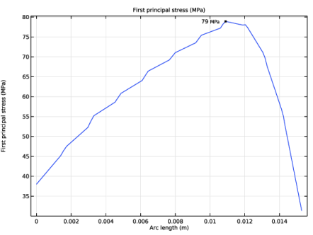
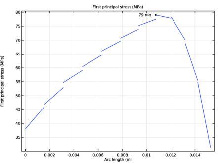
In the Settings window for Line Graph, click Replace Expression in the upper-right corner of the y-Axis Data section. From the menu, choose Component 1 (comp1) > Solid Mechanics > Stress > Principal stresses > solid.sp1Gp - First principal stress - N/m².
4
In the Stress Along Fillet toolbar, click  Plot.
Graph Marker 1
1
Right-click Line Graph 1 and choose Graph Marker.
2
In the Settings window for Graph Marker, locate the Display section.
3
From the Display list, choose Max.
4
Locate the Text Format section. Select the Include unit checkbox.
5
In the Precision text field, type 2.
6
Click to expand the Coloring and Style section. From the Anchor point list, choose Middle right.
7
In the Stress Along Fillet toolbar, click  Plot.
You can get an indication of the discretization errors by switching off the averaging between adjacent elements.
Line Graph 1
1
In the Model Builder window, click Line Graph 1.
2
In the Settings window for Line Graph, click to expand the Quality section.
3
From the Evaluation settings list, choose Manual.
4
From the Smoothing list, choose None.
5
In the Stress Along Fillet toolbar, click  Plot.
Now, assume that the bracket is made from cast iron, a material that is much stronger in compression than in tension. The von Mises criterion, which is isotropic with respect to the stress direction is not suitable in this case. By adding a Safety node, it is possible to check the margins against failure for many different types of materials.
Solid Mechanics (solid)
Linear Elastic Material 1
In the Model Builder window, under Component 1 (comp1) > Solid Mechanics (solid) click Linear Elastic Material 1.
Safety 1
1
In the Physics toolbar, click  Attributes and choose Safety.
The Rankine criterion is suitable for materials where the failure is governed by either the most positive or most negative stress.
2
In the Settings window for Safety, locate the Failure Model section.
3
From the Failure criterion list, choose Rankine.
Here, you can choose to either augment the Structural Steel node under Materials or enter the strength values directly in the Safety node. When a single material is used, it does not matter. When there are several materials in a model, it is a good practice to use the From material option.
4
From the σts list, choose User defined. In the associated text field, type 100[MPa].
5
From the σcs list, choose User defined. In the associated text field, type 400[MPa].
Evaluating safety factors can be done without recomputing the solution. The new variables defined by the recently added Safety node must, however, be made part of the solution. For this, you use Update Solution, which is much faster than actually solving.
Study 1
In the Study toolbar, click  Update Solution.
Results
Stress (solid)
After updating the solution, a new plot has been added to Result Templates.
Result Templates
1
In the Home toolbar, click  Result Templates to open the Result Templates window.
2
Go to the Result Templates window.
3
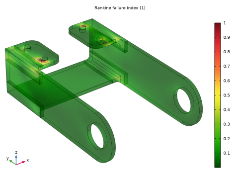
In the tree, select Study 1/Solution 1 (sol1) > Solid Mechanics > Failure Indices (solid) > Failure Index (Safety 1).
4
Click the Add Result Template button in the window toolbar.
5
In the Results toolbar, click  Result Templates to close the Result Templates window.
Results
Surface 1
1
In the Model Builder window, expand the Failure Index (Safety 1) node, then click Surface 1.
2
In the Settings window for Surface, click to expand the Range section.
3
Select the Manual color range checkbox.
4
In the Maximum text field, type 1.
Failure Index (Safety 1)
1
In the Model Builder window, click Failure Index (Safety 1).
2
In the Settings window for 3D Plot Group, locate the Plot Settings section.
3
From the View list, choose New view.
4
In the Failure Index (Safety 1) toolbar, click  Plot.
5
Click the  Show Grid button in the Graphics toolbar.
6
Click the  Scene Light button in the Graphics toolbar.
7
Click the  Transparency button in the Graphics toolbar.
8
In the Failure Index (Safety 1) toolbar, click  Plot.
Finally, check that the total reaction forces and moments match the applied loads.
Result Templates
1
In the Home toolbar, click  Result Templates to open the Result Templates window.
2
Go to the Result Templates window.
3
In the tree, select Study 1/Solution 1 (sol1) > Solid Mechanics > Total Reaction Forces and Moments (Solid Mechanics).
4
Click the Add Result Template button in the window toolbar.
Results
Total Reaction Forces and Moments (Solid Mechanics)
1
In the Total Reaction Forces and Moments (Solid Mechanics) toolbar, click  Evaluate.
Compute the applied moment around the Y-axis.
2
In the Model Builder window, under Results click Total Reaction Forces and Moments (Solid Mechanics).
Distance Measurement 1
1
In the Total Reaction Forces and Moments (Solid Mechanics) toolbar, click  Measure and choose Distance Measurement.
2
3
In the Total Reaction Forces and Moments (Solid Mechanics) toolbar, click  Evaluate.
Global Evaluation 2
1
Right-click Total Reaction Forces and Moments (Solid Mechanics) and choose Global Evaluation.
2
In the Settings window for Global Evaluation, locate the Expressions section.
3
4
In the Total Reaction Forces and Moments (Solid Mechanics) toolbar, click  Evaluate.
Stress (solid)
Click the  Zoom Extents button in the Graphics toolbar.