PDF

Bracket — Shell Analysis
Introduction
The various examples based on a bracket geometry form a suite of tutorials which summarizes the fundamentals when modeling structural mechanics problems in COMSOL Multiphysics and the Structural Mechanics Module.
In this example you study the stress in a bracket subjected to external loads. The thin parts with constant thickness are modeled using the Shell interface, and the transition regions where 3D effects are important are modeled using the Solid Mechanics interface. This example also shows how to connect shell elements with solid elements.
For thin geometries, it can be more efficient to use shell elements than solid elements, thus saving computational time and memory. The Shell interface in the Structural Mechanics Module can be used to model structures approximated by thin or thick shells. There is also a similar Plate interface for 2D problems. The thickness of the shell or plate is taken into account in the equations instead of being explicitly modeled in the geometry.
It is recommended that you review the Introduction to the Structural Mechanics Module, which includes background information and discusses the bracket_basic.mph model relevant to this example.
Model Definition
The model is described in the section “The Fundamentals: A Static Linear Analysis” in the Introduction to the Structural Mechanics Module.
The parts of the geometry modeled with shells are highlighted in Figure 1 and the parts modeled with solids are highlighted in Figure 2.
Figure 1: Shell domains in the bracket geometry.
Figure 2: Solid domains in the bracket geometry.
The load is the same as in the solid model which forms the basis, but is now applied along the edges at the bracket holes.
Results and Discussion
The Shell interface generates a plot which indicates the physical location of top and bottom surfaces. Especially when working with offsets, as in the current example, this is an excellent tool for checking that the input data is correct. This plot is shown in Figure 3.
Figure 3: The shell geometry plot. Red indicates top surface and blue indicates bottom surface.
In another plot, also available under Result Templates, the thickness is indicated by color contours, and the directions of the shell local coordinate systems are shown. This plot is shown in Figure 4.
Figure 4: Plot of thickness and local directions. The Red-Green-Blue convention is used for ordering of the coordinate axes.
There are several types of automatic connections available in the Shell interface. When using such features, it is recommended that you inspect that the connections have been applied as intended. In Figure 5, such a plot is shown. It indicates the boundaries of the solid that are connected to shell elements.
Figure 5: Generated connections between shell and solid elements.
Figure 6 shows the first principal strain in both the solid domains and in the shells. When using the Shell dataset, the shell is represented by a solid with thickness and offset taken from the Shell interface. The through-thickness representation of, for example, stresses is also full 3D. You can increase the resolution of the evaluation in the thickness direction, but using a high resolution may give slower plotting.
As can be seen, the continuity over the transition between the shell and the solid is very good.
Figure 6: First principal strain distribution in the solid and at the top and bottom of the shell.
A special result type in the shell elements are the section forces. The section forces contain the stresses integrated through the thickness of the shell and represent three fundamental types of action:
Membrane (shell.Nl11, shell.Nl22, and shell.Nl12)
Bending (shell.Ml11, shell.Ml22, and shell.Ml12)
Out-of-plane shear (shell.Ql1 and shell.Ql2)
The section forces are always aligned with the shell local system.
As an example of section forces, they evaluated along a cut line through the left arm of the bracket, shown in Figure 7. In this cross section, it is reasonable to expect that the stress state is similar to that of a rectangular beam, subjected to a transverse force at the hole location.
In order to know which components of the section force to study, the local directions can be examined in Figure 4. The first direction is the one along the arm, so shell.Nl11 corresponds to the bending stresses in a beam and shell.Nl12 corresponds to the shear stresses.
Figure 7: The cut line used for examining the section forces.
The relevant membrane forces along the cut are shown in Figure 8.
Figure 8: Membrane forces along the cut line.
The values can be compared with analytical results according to beam theory. As the cut is located at a distance from the hole center of a = 100 mm, the bending moment is
(1)
The peak bending stress in a rectangular beam is
(2)
where t is the thickness and h is the height. The distribution along the cut should be linear.
The section force is the stress multiplied by the thickness, giving the peak value
(3)
According to beam theory, the shear stress has a parabolic distribution with the peak value
(4)
Thus, the peak value of the shear membrane force is
(5)
As can be seen, the stress state in this part of the structure is very close to that of a beam. Checks like this can be valuable for model verification.
Notes About the COMSOL Implementation
You can specify an offset in the shell definition that the meshed surface is not the same as the midsurface of the real geometry. This is used here, since the external geometrical boundaries are immediately available.
The Solid–Thin Structure Connection multiphysics coupling is used for connecting shell edges to solid boundaries.
Application Library path: Structural_Mechanics_Module/Tutorials/bracket_shell
Application Libraries
1
From the File menu, choose Application Libraries.
2
In the Application Libraries window, select Structural Mechanics Module > Tutorials > bracket_static in the tree.
3
Component 1 (comp1)
Start by removing the results from the loaded model.
1
In the Model Builder window, expand the Component 1 (comp1) node.
Results
Study 1/Solution 1 (sol1)
1
In the Model Builder window, expand the Results > Datasets node.
2
Right-click Results > Datasets > Study 1/Solution 1 (sol1) and choose Delete.
3
Right-click Results > Tables and choose Delete All.
Component 1 (comp1)
Add a Shell interface to the model.
Add Physics
1
In the Home toolbar, click  Add Physics to open the Add Physics window.
2
Go to the Add Physics window.
3
In the tree, select Structural Mechanics > Shell (shell).
4
Click the Add to Component 1 button in the window toolbar.
5
In the Home toolbar, click  Add Physics to close the Add Physics window.
Definitions
Add a number of selections.
Solid
1
In the Definitions toolbar, click  Explicit.
2
In the Settings window for Explicit, type Solid in the Label text field.
3
4
Click the  Zoom Extents button in the Graphics toolbar.
5
Click the  Wireframe Rendering button in the Graphics toolbar.
Shell
1
In the Definitions toolbar, click  Explicit.
2
In the Settings window for Explicit, type Shell in the Label text field.
3
Locate the Input Entities section. From the Geometric entity level list, choose Boundary.
4
5
Click the  Wireframe Rendering button in the Graphics toolbar.
Solid Mechanics (solid)
1
In the Model Builder window, under Component 1 (comp1) click Solid Mechanics (solid).
2
In the Settings window for Solid Mechanics, locate the Domain Selection section.
3
From the Selection list, choose Solid.
Disable not used boundary conditions from the Solid Mechanics interface. Both the loads and constraints will be applied to the shell part. This is just to clean up the Model Builder tree. Since these nodes now have an empty selection, they would not influence the analysis if kept.
4
In the Model Builder window, expand the Solid Mechanics (solid) node.
Boundary Load 1, Fixed Constraint 1
1
In the Model Builder window, under Component 1 (comp1) > Solid Mechanics (solid), Ctrl-click to select Fixed Constraint 1 and Boundary Load 1.
2
Not Used; Applied in Shell Interface
1
In the Settings window for Group, type Not Used; Applied in Shell Interface in the Label text field.
2
Right-click Not Used; Applied in Shell Interface and choose Disable.
Add settings to the Shell interface. Since the mesh is placed on the outer boundary, the location of the midsurface is described by an offset.
Shell (shell)
1
Click the  Wireframe Rendering button in the Graphics toolbar.
2
In the Model Builder window, under Component 1 (comp1) click Shell (shell).
3
In the Settings window for Shell, locate the Boundary Selection section.
4
From the Selection list, choose Shell.
Thickness and Offset 1
1
In the Model Builder window, under Component 1 (comp1) > Shell (shell) click Thickness and Offset 1.
2
In the Settings window for Thickness and Offset, locate the Thickness and Offset section.
3
In the d0 text field, type 8[mm].
4
From the Position list, choose Top surface on boundary.
Fixed Constraint 1
1
In the Physics toolbar, click  Edges and choose Fixed Constraint.
2
In the Settings window for Fixed Constraint, locate the Edge Selection section.
3
From the Selection list, choose Bolt Hole Edges.
Edge Load 1
1
In the Physics toolbar, click  Edges and choose Edge Load.
2
In the Settings window for Edge Load, locate the Coordinate System Selection section.
3
From the Coordinate system list, choose Cylindrical System 2 (sys2).
4
5
Locate the Force section. From the Load type list, choose Force per reference area.
6
Specify the fA vector as
Multiphysics
Add the connection between the shells and the solids.
Solid–Thin Structure Connection 1 (sshc1)
1
In the Physics toolbar, click  Multiphysics Couplings and choose Global > Solid–Thin Structure Connection.
2
In the Settings window for Solid–Thin Structure Connection, locate the Connection Settings section.
3
Select the Manual control of selections checkbox.
4
5
From the Method list, choose Flexible.
6
Click the  Wireframe Rendering button in the Graphics toolbar.
Materials
The current material is attached only to the domains. A separate material definition is needed for the boundaries where the Shell interface is active.
Structural steel 1 (mat2)
1
In the Model Builder window, expand the Component 1 (comp1) > Materials node.
2
Right-click Component 1 (comp1) > Materials > Structural steel (mat1) and choose Duplicate.
3
In the Settings window for Material, locate the Geometric Entity Selection section.
4
From the Geometric entity level list, choose Boundary.
5
From the Selection list, choose Shell.
Study 1
Run the analysis.
In the Study toolbar, click  Compute.
Results
Stress (solid)
The default plot for the Shell interface shows the von Mises stress using a Shell dataset. Create a combined stress plot with the results from both interfaces by copying the default stress plot for the solid.
Volume 1
1
In the Model Builder window, expand the Stress (solid) node.
2
Right-click Volume 1 and choose Copy.
Stress, Solid + Shell
1
In the Model Builder window, under Results click Stress (shell).
2
In the Settings window for 3D Plot Group, type Stress, Solid + Shell in the Label text field.
Volume 1
1
Right-click Stress, Solid + Shell and choose Paste Volume.
2
In the Settings window for Volume, click to expand the Inherit Style section.
3
From the Plot list, choose Surface 1.
4
Locate the Data section. From the Dataset list, choose Study 1/Solution 1 (sol1).
Surface 1
1
In the Model Builder window, click Surface 1.
2
In the Settings window for Surface, click to expand the Range section.
3
Select the Manual color range checkbox.
4
In the Maximum text field, type 70.
5
In the Stress, Solid + Shell toolbar, click  Plot.
Add plots from Result Templates, showing the shell geometry, the thickness and local shell system orientation, and the solid-shell connections. The first plot shows the top surface in red and the bottom surface in blue.
Result Templates
1
In the Results toolbar, click  Result Templates to open the Result Templates window.
2
Go to the Result Templates window.
3
In the tree, select Study 1/Solution 1 (sol1) > Shell > Shell Geometry (shell).
4
Click the Add Result Template button in the window toolbar.
5
In the tree, select Study 1/Solution 1 (sol1) > Shell > Thickness and Orientation (shell).
6
Click the Add Result Template button in the window toolbar.
7
In the tree, select Study 1/Solution 1 (sol1) > Solid–Thin Structure Connection 1 > Connected Region Indicator (sshc1).
8
Click the Add Result Template button in the window toolbar.
9
In the Results toolbar, click  Result Templates to close the Result Templates window.
Results
Shell Geometry (shell)
1
In the Shell Geometry (shell) toolbar, click  Plot.
2
Click the  Zoom Extents button in the Graphics toolbar.
Thickness and Orientation (shell)
1
In the Model Builder window, click Thickness and Orientation (shell).
2
In the Thickness and Orientation (shell) toolbar, click  Plot.
Connected Region Indicator (sshc1)
1
In the Model Builder window, click Connected Region Indicator (sshc1).
2
In the Connected Region Indicator (sshc1) toolbar, click  Plot.
Create a plot of the maximum principal stresses.
Principal Strain
1
In the Model Builder window, right-click Stress, Solid + Shell and choose Duplicate.
2
In the Settings window for 3D Plot Group, type Principal Strain in the Label text field.
Surface 1
1
In the Model Builder window, expand the Principal Strain node, then click Surface 1.
2
In the Settings window for Surface, locate the Expression section.
3
In the Expression text field, type shell.ep1.
4
Locate the Range section. In the Maximum text field, type 2.0E-4.
5
Locate the Coloring and Style section. From the Color table type list, choose Discrete.
Volume 1
1
In the Model Builder window, click Volume 1.
2
In the Settings window for Volume, locate the Expression section.
3
In the Expression text field, type solid.ep1.
4
Click the  Zoom Extents button in the Graphics toolbar.
5
In the Principal Strain toolbar, click  Plot.
Create a cut line, and plot section forces along it.
Cut Line 3D 1
1
In the Results toolbar, click  Cut Line 3D.
2
In the Settings window for Cut Line 3D, locate the Line Data section.
3
In row Point 1, set X to -0.215/2.
4
In row Point 2, set X to -0.215/2.
5
In row Point 1, set Y to -0.2.
6
In row Point 2, set Y to -0.2.
7
In row Point 1, set Z to -0.1.
8
In row Point 2, set Z to 0.1.
9
From the Snapping list, choose Snap to closest boundary.
10
Section Forces at Cut
1
In the Results toolbar, click  1D Plot Group.
2
In the Settings window for 1D Plot Group, type Section Forces at Cut in the Label text field.
3
Locate the Data section. From the Dataset list, choose Cut Line 3D 1.
Line Graph 1
1
Right-click Section Forces at Cut and choose Line Graph.
2
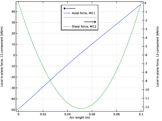
In the Settings window for Line Graph, click Replace Expression in the upper-right corner of the y-Axis Data section. From the menu, choose Component 1 (comp1) > Shell > Section forces > Local in-plane force - N/m > shell.Nl11 - Local in-plane force, 11-component.
3
Locate the y-Axis Data section. From the Unit list, choose kN/m.
4
Click to expand the Legends section. Select the Show legends checkbox.
5
From the Legends list, choose Manual.
6
7
In the Section Forces at Cut toolbar, click  Plot.
Line Graph 2
1
Right-click Line Graph 1 and choose Duplicate.
2
In the Settings window for Line Graph, locate the y-Axis Data section.
3
In the Expression text field, type shell.Nl12.
4
Locate the Legends section. In the table, enter the following settings:
5
In the Section Forces at Cut toolbar, click  Plot.
Section Forces at Cut
1
In the Model Builder window, click Section Forces at Cut.
2
In the Settings window for 1D Plot Group, click to expand the Title section.
3
From the Title type list, choose None.
4
Locate the Plot Settings section. Select the Two y-axes checkbox.
5
In the table, select the Plot on secondary y-axis checkbox for Line Graph 2.
6
Locate the Legend section. From the Position list, choose Upper middle.
7
In the Section Forces at Cut toolbar, click  Plot.