COMSOL 6.4 - Bracket — Reduced-Order Modeling

Transient analyses provide the time-domain response of a structure subjected to time-dependent loads. Solving large models in time domain may be computationally intensive in terms of memory and CPU time. Modal reduced-order modeling is one approach available to improve the performance for linear structural dynamics.

In this example you learn how to create a reduced-order model: from defining the model inputs and outputs, setting up the model reduction study, and finally postprocessing the reconstructed solution on the full geometry.

It is recommended you review the model Bracket — Transient Analysis, which includes background information and discusses the models relevant for this example.

Model Definition

The model geometry is represented in Figure 1.

Figure 1: Bracket geometry.

A rigid body is assumed to be connected to the holes in the arms of the bracket. This body is modeled using a rigid connector. Time-varying loads are applied to it.

•

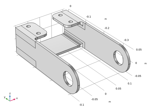
In the x direction, a rectangular pulse train with amplitude 400 N and width 0.5 ms is acting every 10 ms

•

In the y direction, a 500 N force with300 Hz sinusoidal time dependence is acting

•

In the z direction, a constant load of −100 N is applied

In the first stage of this tutorial, you will set up the reduced-order model (ROM) and compare the solution with the results from the unreduced model for a short segment of the start-up transient. In a second stage, you will compute the solution up to steady-state, as the ROM allow much faster computations.

Results and Discussion

Figure 2 shows the rigid connector’s displacements at the center of rotation versus time. The black dotted lines correspond to the solution computed with the unreduced model. This validates the choice for the number of eigenfrequencies and tolerance used by the solver.

Figure 2: Displacement of the pin center of rotation vs time computed with either reduced model (colored solid lines) or unreduced model (black dotted lines).

In Figure 3 below, you can see that the steady state is reached after about 250 ms. This time depends on the chosen damping parameters.

Figure 3: Displacement of the pin center of rotation vs time.

Figure 4 below shows the displacement of the pin center of rotation for the steady state regime only. The bracket arm displacement in both the y and z directions oscillate at the same frequency (300 Hz) as the harmonic excitation in the y direction. The z-direction displacements are also slightly shifted due to the negative constant z-direction load. In the x direction, however, the oscillations are dominated by the first natural frequency. Note also the small dip every 10 ms corresponding to the periodic pulse applied in the x direction.

Figure 4: Displacement of the pin center of rotation versus time, steady state regime only.

In Figure 5, the von Mises stress distribution computed using the unreduced model is compared with the one reconstructed from a reduced model solution for some time steps. The figure shows a good agreement between the two types of solutions.