PDF

Bracket — Parametric Analysis
Introduction
The various examples based on a bracket geometry form a suite of tutorials which summarizes the fundamentals when modeling structural mechanics problems in COMSOL Multiphysics and the Structural Mechanics Module.
This example includes computing the solution to a case where the direction of the load is changed using a parametric sweep over a set of directions.
It is recommended you review the Introduction to the Structural Mechanics Module, which includes background information.
Model Definition
This example is an extension of the one described in the section “The Fundamentals: A Static Linear Analysis” in the Introduction to the Structural Mechanics Module. The same model is also available as a standalone model in the Application Libraries as Bracket - Static Analysis.
The geometry is shown in Figure 1.
Figure 1: Bracket geometry.
In this analysis, the mounting bolts are assumed to be fixed and securely bonded to the bracket. To model the external load from the pin, you specify a surface load p with a trigonometric distribution on the inner surfaces of the two holes:
where p0 is the peak load intensity. The main direction of the load is defined by θ0, the angle from the y-axis. The load on the two holes acts in opposite directions. The orientation of the load is controlled by a local coordinate system with axis directions generated using the sweep parameter theta0.
Results
Figure 2 shows the von Mises stress distribution corresponding to a twisting load case, where the load acts in the positive z direction in the left arm and in the negative z direction in the right arm.
Figure 2: Von Mises stress in a twisting load case (parameter theta0 = 0°).
Figure 3 shows the von Mises stress distribution corresponding of a tensile load in the right arm and a compressive load in the left arm. The maximum von Mises stress value is significantly lower in this case..
Figure 3: Von Mises stress in a tensile and compressive load case (parameter theta0 = 90°).
Figure 4 shows the von Mises stress distribution corresponding to a load orientation of 130°.
Figure 4: Von Mises stress for parameter theta0 = 130°.
The reaction forces at the first bolt location are shown in Figure 5. It should be noted that for a pretensioned bolt connection, this cannot be directly interpreted as the bolt force. In such a case, the force distribution in the bolts is far more complex. Only if the bracket is connected to its surrounding by rivets, or loosely tightened bolts, this result reflects the actual forces in the joint element.
Figure 5: Forces at the first attachment point as function of the load angle
Finally, the variation of the stress with the load angle in some points is studied in Figure 6. It is clear that the load angles that induce a bending/twisting state cause higher stresses than those which give predominantly tension and compression.
Figure 6: von Mises stress as function of the load angle for three different high stress locations.
Notes About the COMSOL Implementation
In COMSOL Multiphysics, you have two ways to perform parametric studies — using either a Parametric Sweep node or the Auxiliary sweep from the Stationary Solver node. In this example, either method can be used. An Auxiliary sweep is used here, but the continuation solver is not used. The continuation solver uses the solution from the previous parameter as an initial guess to calculate the current parameter value, which is the preferred option for nonlinear problems. Using the Parametric Sweep node is necessary for applications requiring, for example, geometric parameterization.
It can be noted that the stiffness matrix in this case is only inverted once. The solver automatically recognizes the fact that it is only the loads, and thus the right hand side of the system of equations, that are changing between the parameter steps.
Application Library path: Structural_Mechanics_Module/Tutorials/bracket_parametric
Parametric studies can be set up from scratch or, as in this example, added to an existing study.
Application Libraries
1
From the File menu, choose Application Libraries.
2
In the Application Libraries window, select Structural Mechanics Module > Tutorials > bracket_static in the tree.
3
Global Definitions
In this model, the stress in the bracket is computed for different load orientations. First add a parameter to set the load direction angle.
Parameters 1
1
In the Model Builder window, under Global Definitions click Parameters 1.
2
In the Settings window for Parameters, locate the Parameters section.
3
Component 1 (comp1)
Let the reference orientation of the cylindrical system rotate with the load orientation
1
In the Model Builder window, expand the Component 1 (comp1) node.
Definitions
Cylindrical System 2 (sys2)
1
In the Model Builder window, expand the Component 1 (comp1) > Definitions node, then click Cylindrical System 2 (sys2).
2
In the Settings window for Cylindrical System, locate the Settings section.
3
Find the Direction of axis ϕ=0 subsection. In the table, enter the following settings:
Left Pin Hole
Since the load is rotating inside the holes, it is no longer sufficient that half of the holes are selected.
1
In the Model Builder window, expand the Component 1 (comp1) > Definitions > Selections node, then click Left Pin Hole.
2
In the Settings window for Explicit, locate the Input Entities section.
3
Select the Group by continuous tangent checkbox.
Right Pin Hole
1
In the Model Builder window, click Right Pin Hole.
2
In the Settings window for Explicit, locate the Input Entities section.
3
Select the Group by continuous tangent checkbox.
Solid Mechanics (solid)
Since the entire circumference of each hole is now selected, the expression for the pressure must be truncated so that it acts only on the intended 180 degrees.
Boundary Load 1
1
In the Model Builder window, expand the Component 1 (comp1) > Solid Mechanics (solid) node, then click Boundary Load 1.
2
In the Settings window for Boundary Load, locate the Force section.
3
Specify the fA vector as
Study 1
Add an auxiliary sweep parameter, and compute the results.
Step 1: Stationary
1
In the Model Builder window, expand the Study 1 node, then click Step 1: Stationary.
2
In the Settings window for Stationary, click to expand the Study Extensions section.
3
Select the Auxiliary sweep checkbox.
4
5
6
From the Run continuation for list, choose No parameter.
7
In the Study toolbar, click  Compute.
Results
Stress (solid)
The default plot shows the solution for the last parameter value (160[deg]). You can easily change the parameter value to display the plot and then compare solutions for different load cases.
The following instructions reproduce Figure 2 to Figure 4.
1
In the Settings window for 3D Plot Group, click  Plot First.
2
Locate the Data section. From the Parameter value (theta0 (deg)) list, choose 90.
3
In the Stress (solid) toolbar, click  Plot.
4
From the Parameter value (theta0 (deg)) list, choose 130.
5
In the Stress (solid) toolbar, click  Plot.
Force in Bolt 1
You will now create a plot showing how the reaction forces vary with the load angle.
1
In the Results toolbar, click  Evaluation Group.
2
In the Settings window for Evaluation Group, type Force in Bolt 1 in the Label text field.
Surface Integration 1
1
Right-click Force in Bolt 1 and choose Integration > Surface Integration.
2
In the Settings window for Surface Integration, locate the Selection section.
3
From the Selection list, choose Bolt 1.
4
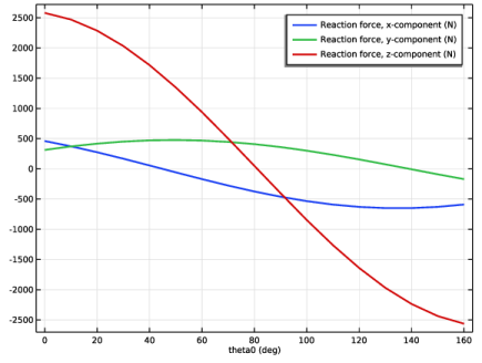
Click Replace Expression in the upper-right corner of the Expressions section. From the menu, choose Component 1 (comp1) > Solid Mechanics > Reactions > Reaction force (spatial frame) - N > All expressions in this group.
5
In the Force in Bolt 1 toolbar, click  Evaluate.
Force in Bolt 1
1
Go to the Force in Bolt 1 window.
2
Click the Table Graph button in the window toolbar.
Results
Table Graph 1
1
In the Settings window for Table Graph, click to expand the Legends section.
2
Select the Show legends checkbox.
3
Locate the Coloring and Style section. From the Width list, choose 2.
4
In the 1D Plot Group 7 toolbar, click  Plot.
Create a graph of how the stress varies with the load angle in some interesting points.
Force in Bolt 1
1
In the Model Builder window, under Results click 1D Plot Group 7.
2
In the Settings window for 1D Plot Group, type Force in Bolt 1 in the Label text field.
Stress as Function of Load Angle
1
In the Results toolbar, click  1D Plot Group.
2
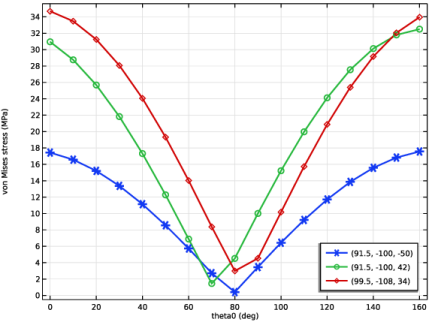
In the Settings window for 1D Plot Group, type Stress as Function of Load Angle in the Label text field.
Point Graph 1
1
Right-click Stress as Function of Load Angle and choose Point Graph.
2
3
In the Settings window for Point Graph, locate the y-Axis Data section.
4
In the Expression text field, type solid.mises.
5
Click to expand the Coloring and Style section. From the Width list, choose 2.
6
Find the Line markers subsection. From the Marker list, choose Cycle.
Annotate the graphs by the location of each point.
7
Click to expand the Legends section. Select the Show legends checkbox.
8
From the Legends list, choose Evaluated.
9
In the Legend text field, type (eval(X,mm), eval(Y,mm), eval(Z,mm)).
10
In the Stress as Function of Load Angle toolbar, click  Plot.
Stress as Function of Load Angle
1
In the Model Builder window, click Stress as Function of Load Angle.
2
In the Settings window for 1D Plot Group, click to expand the Title section.
3
From the Title type list, choose None.
4
Locate the Legend section. From the Position list, choose Lower right.
5
In the Stress as Function of Load Angle toolbar, click  Plot.