PDF

Bracket — Inertia Relief Analysis
Introduction
The various examples based on a bracket geometry form a suite of tutorials summarizing the fundamentals of modeling structural mechanics problems in COMSOL Multiphysics and the Structural Mechanics Module.
In this example, you learn how to perform an inertia relief analysis. This type of analysis is intended for situations where an unconstrained structure is accelerated by external forces. The applied loads and the inertial forces caused by the acceleration will then be in balance. This type of analysis is common in, for example, aerospace engineering.
From an engineering point of view, analyzing the behavior of an unconstrained bracket can be of little interest. Thus, the purpose of this example is just to demonstrate how to set up an inertia relief analysis.
It is recommended that you review the Introduction to the Structural Mechanics Module, which includes relevant background information.
In the Structural Mechanics Modeling chapter of the Structural Mechanics Module User’s Guide: Inertia Relief Study.
Model Definition
The model used in this guide is a bracket made of steel. Figure 1 shows the geometry.
Figure 1: Bracket geometry.
In this analysis, the bracket is unconstrained. One of the arms is loaded upward and the other downward. The loads are applied as total forces of 65 N, acting in opposite directions on the inner surfaces of the holes.
Results
Figure 2 shows the von Mises stress distribution together with an exaggerated picture of the deformation.
Figure 2: von Mises stress distribution in the bracket.
It should, however, be noted that the displacement field computed in an inertia relief analysis is not unique; it is relative to an arbitrary rigid-body motion.
Figure 3 shows the acceleration. Since there is no resultant force, the motion mainly consists of a rotational acceleration around the y-axis.
Figure 3: Inertia relief acceleration. The gray sphere in the middle is not part of the structure; it just indicates the location of the center of mass of the bracket.
Notes About the COMSOL Implementation
To perform an inertial relief analysis, you add an Inertia Relief node to the physics interface. In most cases, you do not need to change any settings. You should not use any other types of constraints or elastic supports; the structure must be able to move freely as rigid body.
Then, you click the Create Load Groups and Study button. A special set of load groups will be added, together with a new study. This study consists of two stationary study steps. In the first step, a number of load cases (six in 3D) are solved. Using these load cases, a rigid-body acceleration is determined, using the conditions that the external loads are balanced by inertia forces. In the second study step, the external load and the computed inertia forces are all combined together to form the total solution.
Application Library path: Structural_Mechanics_Module/Tutorials/bracket_inertia_relief
Modeling Instructions
Application Libraries
1
From the File menu, choose Application Libraries.
2
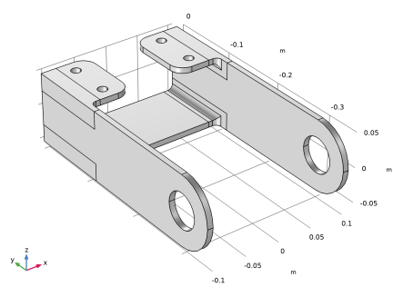
In the Application Libraries window, select Structural Mechanics Module > Tutorials > bracket_basic in the tree.
3
Global Definitions
Parameters 1
1
In the Model Builder window, under Global Definitions click Parameters 1.
2
In the Settings window for Parameters, locate the Parameters section.
3
Solid Mechanics (solid)
Fixed Constraint 1
1
In the Model Builder window, expand the Component 1 (comp1) > Solid Mechanics (solid) node.
2
Right-click Component 1 (comp1) > Solid Mechanics (solid) > Fixed Constraint 1 and choose Delete.
Boundary Load 1
1
In the Physics toolbar, click  Boundaries and choose Boundary Load.
Apply a boundary load to the bracket holes.
2
In the Settings window for Boundary Load, locate the Boundary Selection section.
3
From the Selection list, choose Pin Holes.
4
Locate the Coordinate System Selection section. From the Coordinate system list, choose Boundary System 1 (sys1).
5
Locate the Force section. Specify the fA vector as
Since the entire circumference of each hole is selected, the expression for the pressure must be truncated so that it acts only on the intended 180 degrees.
Inertia Relief 1
1
In the Physics toolbar, click  Domains and choose Inertia Relief.
2
In the Settings window for Inertia Relief, click Automated Model Setup in the upper-right corner of the Inertia Relief section. From the menu, choose Create Load Groups and Study.
Definitions
Mass Properties 1 (mass1)
1
In the Model Builder window, expand the Component 1 (comp1) > Definitions node.
2
Right-click Definitions and choose Physics Utilities > Mass Properties.
3
In the Settings window for Mass Properties, locate the Density section.
4
From the Density source list, choose From physics interface.
Inertia Relief Study
In the Study toolbar, click  Compute.
Results
Stress (solid)
1
In the Settings window for 3D Plot Group, locate the Color Legend section.
2
Select the Show maximum and minimum values checkbox.
Inertia relief acceleration (solid)
1
Right-click Stress (solid) and choose Duplicate.
2
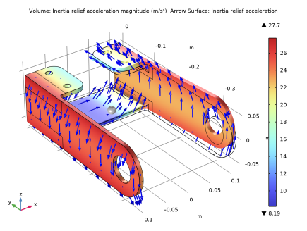
In the Settings window for 3D Plot Group, type Inertia relief acceleration (solid) in the Label text field.
Volume 1
1
In the Model Builder window, expand the Inertia relief acceleration (solid) node, then click Volume 1.
2
In the Settings window for Volume, click Replace Expression in the upper-right corner of the Expression section. From the menu, choose Component 1 (comp1) > Solid Mechanics > Acceleration and velocity > solid.air - Inertia relief acceleration magnitude - m/s².
3
Locate the Coloring and Style section. From the Color table list, choose RainbowLight.
Arrow Surface 1
1
In the Model Builder window, right-click Inertia relief acceleration (solid) and choose Arrow Surface.
2
In the Settings window for Arrow Surface, click Replace Expression in the upper-right corner of the Expression section. From the menu, choose Component 1 (comp1) > Solid Mechanics > Acceleration and velocity > solid.airX,...,solid.airZ - Inertia relief acceleration.
3
Locate the Coloring and Style section. From the Arrow length list, choose Logarithmic.
4
From the Color list, choose Blue.
5
From the Arrow length list, choose Normalized.
6
Select the Scale factor checkbox. In the associated text field, type 0.001.
Inertia relief acceleration (solid)
In the Model Builder window, click Inertia relief acceleration (solid).
Point Trajectories 1
1
In the Inertia relief acceleration (solid) toolbar, click  More Plots and choose Point Trajectories.
2
In the Settings window for Point Trajectories, locate the Coloring and Style section.
3
Find the Line style subsection. From the Type list, choose None.
4
Find the Point style subsection. From the Type list, choose Point.
5
Click Replace Expression in the upper-right corner of the Trajectory Data section. From the menu, choose Component 1 (comp1) > Definitions > Mass Properties 1 > mass1.CMX,...,mass1.CMZ - Center of mass.
6
Click to expand the Title section. From the Title type list, choose None.
7
Locate the Coloring and Style section. In the Point radius expression text field, type 0.008.
8
Select the Radius scale factor checkbox.
9
From the Color list, choose Gray.
10
In the Inertia relief acceleration (solid) toolbar, click  Plot.
11
Click the  Zoom Extents button in the Graphics toolbar.