PDF

Bracket — Explicit Dynamics
Introduction
The various examples based on a bracket geometry form a suite of tutorials which summarizes the fundamentals when modeling structural mechanics problems in COMSOL Multiphysics and the Structural Mechanics Module
In this example, you learn how to set up an explicit structural dynamic analysis by performing a drop test the bracket. Explicit time stepping for structural mechanics is an alternative to the more general implicit methods. It is the preferred choice for certain classes of problems. One example is short duration events with contact such as a drop test.
From an engineering point of view, analyzing a drop test of a bracket can be of little interest. Thus, the purpose of this example is just to demonstrate how to set up an explicit dynamic analysis, highlight good modeling practices, and discuss some additional modeling considerations required as compared to an implicit analysis.
It is recommended that you review the Introduction to the Structural Mechanics Module, which includes relevant background information.
In the Structural Mechanics Modeling chapter of the Structural Mechanics Module User’s Guide:
Model Definition
The model used in this guide is a bracket made of steel. The model geometry is represented in Figure 1. In this example the bracket is dropped from a height of 2 meters on to a rigid surface at an inclined angle, causing a series of impacts between the bracket and the surface.
Figure 1: Bracket geometry.
Results and Discussion
Figure 2 shows the vertical velocity of the bracket at six time instances during the drop test.
Figure 2: History of the vertical velocity in the bracket during the drop test.
A more detailed picture of the variation of the velocity of the two pin holes is shown Figure 3. We can clearly identify the various impacts and how bracket after around 6 milliseconds bounces back.
Figure 3: Vertical velocity of the two pin holes during the drop test.
Figure 3 shows the results obtained from the explicit dynamics analysis, which can be compared to the results from an implicit dynamic analysis, as shown in Figure 4. The results from the two alternative methods are qualitatively in good agreement.
Figure 4: Vertical velocity of the two pin holes during the drop test using implicit time-stepping.
Figure 5 shows the history of the maximum stress in the bracket. Note that the highest value The stress exceeds the yield strength of a standard steel, and a more realistic simulation should then include the effects of material nonlinearity by plastic deformation. Also here, the results from the explicit and implicit methods are in good agreement.
Figure 5: Maximum von Mises stress in the bracket during the event.
Since explicit time-stepping does not require equilibrium of forces to be established to advance the solution, it is good practice to inspect various energy quantities in the model to verify that the results are sound. This becomes extra important for models that includes mass scaling and hourglass stabilization to check that these artificial energies are small. The histories of most important energy quantities are shown in Figure 6. Clearly, the energy contribution from mass scaling and hourglass stabilization is small.
Figure 6: Total energies.
Notes About the COMSOL Implementation
An explicit dynamic analysis is set up by adding the Solid Mechanics, Explicit Dynamics interface and the Explicit Dynamics study. By also adding a Time Dependent study to model, an implicit dynamic analysis is set up for comparison.
The Solid Mechanics, Explicit Dynamics interface only supports a linear discretization order and by default enables reduced integration for all material models. Always make sure that there are not hourglass modes present in the model, and that the energy added by hourglass stabilization is small.
The time step of an explicit dynamic analysis is limited by the mesh and the material properties. To reduce the solution time
Model the impact by an initial velocity. The free fall velocity from height a h is . Simulating the whole fall from the drop height would take an enormous number of time steps.
Application Library path: Structural_Mechanics_Module/Tutorials/bracket_explicit
Modeling Instructions
From the File menu, choose New.
New
In the New window, click  Model Wizard.
Model Wizard
1
In the Model Wizard window, click  3D.
Add a Solid Mechanics, Explicit Dynamics physics interface as a starting point for the explicit dynamics analysis.
2
In the Select Physics tree, select Structural Mechanics > Explicit Dynamics > Solid Mechanics, Explicit Dynamics (solid).
3
Click Add.
To perform a time-domain analysis by explicit time-stepping, use the Explicit Dynamics study step.
4
Click  Study.
5
In the Select Study tree, select Preset Studies for Selected Physics Interfaces > Explicit Dynamics.
6
Geometry 1
Import 1 (imp1)
1
In the Geometry toolbar, click  Import.
2
In the Settings window for Import, locate the Source section.
3
From the Source list, choose COMSOL Multiphysics file.
4
Click  Browse.
5
6
Click  Import.
The Solid Mechanics, Explicit Dynamics interface only supports a linear displacement field. A free tetrahedral mesh should thus be used cautiously due to the poor accuracy of the constant strain tetrahedra. Partition the bracket to facilitate a hex dominant mesh.
7
In the Model Builder window, click Geometry 1.
8
In the Settings window for Geometry, locate the Cleanup section.
9
Clear the Automatic detection of small details checkbox.
Partition Domains 1 (pard1)
1
In the Geometry toolbar, click  Booleans and Partitions and choose Partition Domains.
2
On the object imp1, select Domain 1 only.
3
In the Settings window for Partition Domains, locate the Partition Domains section.
4
From the Partition with list, choose Extended faces.
5
On the object imp1, select Boundaries 9 and 39 only.
6
Click  Build All Objects.
Now create the mesh.
Mesh 1
Swept 1
In the Mesh toolbar, click  Swept.
Size
The time step in explicit dynamics is controlled by the smallest mesh element. Set a stricter restriction on the size distribution of mesh elements created for the bracket.
1
In the Model Builder window, click Size.
2
In the Settings window for Size, locate the Element Size section.
3
Click the Custom button.
4
Locate the Element Size Parameters section. In the Maximum element size text field, type 5[mm].
5
In the Minimum element size text field, type 4[mm].
6
In the Curvature factor text field, type 0.8.
7
In the Resolution of narrow regions text field, type 0.3.
8
Click  Build All.
Inspect the quality of the built mesh using the Cell time result template. It shows a fraction of the mesh elements with the smallest cell time to indicate what regions of the mesh to improve. First add material properties.
Add Material
1
In the Materials toolbar, click  Add Material to open the Add Material window.
2
Go to the Add Material window.
3
In the tree, select Built-in > Structural steel.
4
Click the Add to Component button in the window toolbar.
5
In the Materials toolbar, click  Add Material to close the Add Material window.
Study 1
In the Study toolbar, click  Get Initial Value.
Result Templates
1
In the Home toolbar, click  Windows and choose Result Templates.
2
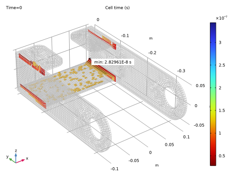
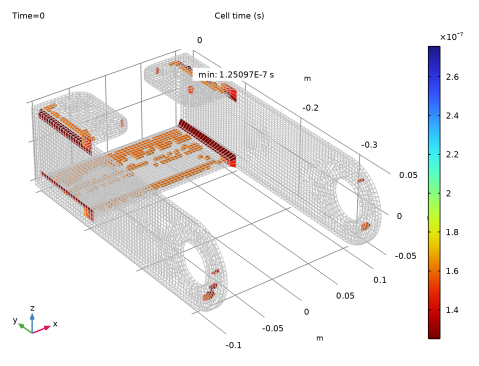
Go to the Result Templates window.
3
In the tree, select Study 1/Solution 1 (sol1) > Solid Mechanics, Explicit Dynamics > Cell Time (solid).
4
Click the Add Result Template button in the window toolbar.
Results
Cell Time (solid)
The mesh close to the fillets can clearly be improved. Partition the bracket further.
Geometry 1
Work Plane 1 (wp1)
1
In the Geometry toolbar, click  Work Plane.
2
In the Settings window for Work Plane, locate the Plane Definition section.
3
From the Plane list, choose zx-plane.
4
From the Offset type list, choose Through vertex.
5
On the object pard1, select Point 17 only.
Partition Domains 2 (pard2)
1
In the Geometry toolbar, click  Booleans and Partitions and choose Partition Domains.
2
On the object pard1, select Domains 1 and 5 only.
Work Plane 2 (wp2)
1
In the Geometry toolbar, click  Work Plane.
2
In the Settings window for Work Plane, locate the Plane Definition section.
3
From the Offset type list, choose Through vertex.
4
On the object pard2, select Point 18 only.
Partition Domains 3 (pard3)
1
In the Geometry toolbar, click  Booleans and Partitions and choose Partition Domains.
2
On the object pard2, select Domains 2 and 7 only.
Work Plane 3 (wp3)
1
In the Geometry toolbar, click  Work Plane.
2
In the Settings window for Work Plane, locate the Plane Definition section.
3
From the Offset type list, choose Through vertex.
4
On the object pard3, select Point 19 only.
Partition Domains 4 (pard4)
1
In the Geometry toolbar, click  Booleans and Partitions and choose Partition Domains.
2
On the object pard3, select Domains 2 and 8 only.
Work Plane 4 (wp4)
1
In the Geometry toolbar, click  Work Plane.
2
In the Settings window for Work Plane, locate the Plane Definition section.
3
From the Plane list, choose yz-plane.
4
From the Offset type list, choose Through vertex.
5
On the object pard4, select Point 31 only.
Partition Domains 5 (pard5)
1
In the Geometry toolbar, click  Booleans and Partitions and choose Partition Domains.
2
On the object pard4, select Domains 5 and 6 only.
Work Plane 5 (wp5)
1
In the Geometry toolbar, click  Work Plane.
2
In the Settings window for Work Plane, locate the Plane Definition section.
3
From the Plane list, choose yz-plane.
4
From the Offset type list, choose Through vertex.
5
On the object pard5, select Point 71 only.
Partition Domains 6 (pard6)
1
In the Geometry toolbar, click  Booleans and Partitions and choose Partition Domains.
2
On the object pard5, select Domains 7 and 9 only.
Partition Edges 1 (pare1)
1
In the Geometry toolbar, click  Booleans and Partitions and choose Partition Edges.
2
On the object pard6, select Edges 54 and 134 only.
Work Plane 6 (wp6)
1
In the Geometry toolbar, click  Work Plane.
2
In the Settings window for Work Plane, locate the Plane Definition section.
3
From the Plane list, choose yz-plane.
4
From the Offset type list, choose Through vertex.
5
On the object pare1, select Point 28 only.
Partition Domains 7 (pard7)
1
In the Geometry toolbar, click  Booleans and Partitions and choose Partition Domains.
2
On the object pare1, select Domains 5 and 6 only.
Work Plane 7 (wp7)
1
In the Geometry toolbar, click  Work Plane.
2
In the Settings window for Work Plane, locate the Plane Definition section.
3
From the Plane list, choose yz-plane.
4
On the object pard7, select Point 84 only.
5
From the Offset type list, choose Through vertex.
6
On the object pard7, select Point 84 only.
Partition Domains 8 (pard8)
1
In the Geometry toolbar, click  Booleans and Partitions and choose Partition Domains.
2
On the object pard7, select Domains 12 and 13 only.
Mesh Control Domains 1 (mcd1)
1
In the Geometry toolbar, click  Virtual Operations and choose Mesh Control Domains.
2
On the object fin, select Domains 5–15 only.
3
In the Geometry toolbar, click  Build All.
Also update the mesh sequence.
Mesh 1
Mapped 1
1
In the Mesh toolbar, click  More Generators and choose Mapped.
2
3
Distribution 1
1
Right-click Mapped 1 and choose Distribution.
2
3
In the Settings window for Distribution, locate the Distribution section.
4
In the Number of elements text field, type 1.
Swept 2
1
In the Mesh toolbar, click  Swept.
2
In the Settings window for Swept, locate the Domain Selection section.
3
From the Geometric entity level list, choose Domain.
4
Distribution 1
1
Right-click Swept 2 and choose Distribution.
2
In the Settings window for Distribution, locate the Distribution section.
3
In the Number of elements text field, type 3.
4
Click  Build All.
Do Get Initial Value to inspect the improved mesh.
Study 1
In the Study toolbar, click  Get Initial Value.
Results
Cell Time (solid)
1
In the Model Builder window, under Results click Cell Time (solid).
The smallest cell time of the new mesh is increased by more than a factor 5. Since the solution time is inversely proportional to the allowed time step, you have thus effectively also reduced solution time by a factor 5.
Now you can finalize the set up of the problem. Start by rotating the bracket to induce an inclined impact.
Geometry 1
Rotate 1 (rot1)
1
In the Geometry toolbar, click  Transforms and choose Rotate.
2
3
In the Settings window for Rotate, locate the Rotation section.
4
From the Specify list, choose Euler angles (Z-X-Z).
5
In the α text field, type 10.
6
In the β text field, type -10.
7
In the γ text field, type -10.
Add a surface for the bracket to impact.
Block 1 (blk1)
1
In the Geometry toolbar, click  Block.
2
In the Settings window for Block, locate the Size and Shape section.
3
In the Height text field, type 0.05.
4
Locate the Position section. From the Base list, choose Center.
5
In the x text field, type 0.1.
6
In the y text field, type -0.1.
7
In the z text field, type -0.025.
The bracket is dropped from a height of 2 meters. However, since the time step size in explicit dynamics is small, it is costly to include the free fall. Move the bracket close to the surface and use an initial velocity equal to the expected free fall velocity.
Move 1 (mov1)
1
In the Geometry toolbar, click  Transforms and choose Move.
2
3
In the Settings window for Move, locate the Displacement section.
4
From the Specify list, choose Positions.
5
Click to select the  Activate Selection toggle button for Vertex to move.
6
On the object rot1, select Point 10 only.
7
From the New position list, choose Coordinates.
8
In the z text field, type 1[mm].
9
Click  Build All Objects.
Define the initial velocity of the bracket.
Solid Mechanics, Explicit Dynamics (solid)
Initial Values 1
1
In the Model Builder window, under Component 1 (comp1) > Solid Mechanics, Explicit Dynamics (solid) click Initial Values 1.
2
In the Settings window for Initial Values, locate the Initial Values section.
3
In the Structural velocity field vector, enter
Only the bracket needs to be included in the physics.
4
In the Model Builder window, click Solid Mechanics, Explicit Dynamics (solid).
5
Add a Contact Pair to define the interaction between the bracket and the rigid surface.
Definitions
Contact Pair 1 (p1)
1
In the Definitions toolbar, click  Pairs and choose Contact Pair.
2
3
In the Settings window for Pair, locate the Destination Boundaries section.
4
Click to select the  Activate Selection toggle button.
5
Set up contact properties, including friction.
Solid Mechanics, Explicit Dynamics (solid)
Contact 1
1
In the Model Builder window, under Component 1 (comp1) > Solid Mechanics, Explicit Dynamics (solid) click Contact 1.
2
In the Settings window for Contact, locate the Contact Pressure Penalty Factor section.
3
From the Penalty factor control list, choose Manual tuning.
4
In the fp text field, type 0.1.
5
Find the Penalty function subsection. From the list, choose Smooth ramp.
Friction 1
1
In the Physics toolbar, click  Attributes and choose Friction.
2
In the Settings window for Friction, locate the Friction Parameters section.
3
In the μ text field, type 0.3.
4
Locate the Friction Force Penalty Factor section. From the Penalty factor control list, choose From parent.
Gravity 1
1
In the Physics toolbar, click  Global and choose Gravity.
While the bracket is affected by gravity forces also during and after the impact, its effects are small and could be omitted. For explicit dynamics, this can save some computational time since the cost to assemble body forces is not negligible.
From the Cell time plot, it was apparent that the time step is still limited by mesh elements at the fillets. You could continue to improve the mesh. This is, however, not straightforward. Since the time step is also proportional to the mass, an alternative is to increase the mass of the smallest mesh elements. This can be done by adding a Mass Scaling node.
Mass Scaling 1
1
In the Physics toolbar, click  Domains and choose Mass Scaling.
2
In the Settings window for Mass Scaling, locate the Domain Selection section.
3
From the Selection list, choose All domains.
Select a target cell time that limits the additional mass to mesh element around the fillets. It is good practice to verify the amount of added mass and its effect. The mass in itself can be checked using an initial value solution. The extra kinetic energy that it causes can be monitored a posteriori.
4
Locate the Mass Scaling section. In the Δtcell0 text field, type 1.5e-7.
The block representing the rigid surface can be meshed by a single mesh element.
Mesh 1
Mapped 2
1
In the Mesh toolbar, click  More Generators and choose Mapped.
2
3
Distribution 1
1
Right-click Mapped 2 and choose Distribution.
2
In the Settings window for Distribution, locate the Distribution section.
3
In the Number of elements text field, type 1.
4
Locate the Edge Selection section. From the Selection list, choose All edges.
Distribution 1
1
In the Model Builder window, right-click Swept 1 and choose Distribution.
2
3
In the Settings window for Distribution, locate the Distribution section.
4
In the Number of elements text field, type 1.
Run the study step for 10 milliseconds.
Study 1
Step 1: Explicit Dynamics
1
In the Model Builder window, under Study 1 click Step 1: Explicit Dynamics.
2
In the Settings window for Explicit Dynamics, locate the Study Settings section.
3
From the Time unit list, choose ms.
4
In the Output times text field, type range(0,0.2,10).
5
Click to expand the Results While Solving section. Select the Plot checkbox.
Set default units for result presentation, verify the mass added by the Mass Scaling node and modify the previously created default stress plot.
6
In the Study toolbar, click  Get Initial Value.
Results
Preferred Units 1
1
In the Results toolbar, click  Configurations and choose Preferred Units.
2
In the Settings window for Preferred Units, locate the Units section.
3
Click  Add Physical Quantity.
4
In the Physical Quantity dialog, select General > Displacement (m) in the tree.
5
6
In the Settings window for Preferred Units, locate the Units section.
7
8
Click  Add Physical Quantity.
9
In the Physical Quantity dialog, select Solid Mechanics > Stress tensor (N/m^2) in the tree.
10
11
In the Settings window for Preferred Units, locate the Units section.
12
13
Click  Apply.
Evaluation Group 1
1
In the Results toolbar, click  Evaluation Group.
2
In the Settings window for Evaluation Group, locate the Data section.
3
From the Time selection list, choose First.
Volume Integration 1
1
Right-click Evaluation Group 1 and choose Integration > Volume Integration.
2
3
In the Settings window for Volume Integration, click Replace Expression in the upper-right corner of the Expressions section. From the menu, choose Component 1 (comp1) > Solid Mechanics, Explicit Dynamics > Material properties > solid.rhoa - Artificial density - kg/m³.
4
Locate the Expressions section. In the table, enter the following settings:
Volume Integration 2
1
Right-click Volume Integration 1 and choose Duplicate.
2
In the Settings window for Volume Integration, click Replace Expression in the upper-right corner of the Expressions section. From the menu, choose Component 1 (comp1) > Solid Mechanics, Explicit Dynamics > Material properties > solid.rho - Density - kg/m³.
3
Locate the Expressions section. In the table, enter the following settings:
Evaluation Group 1
1
In the Model Builder window, click Evaluation Group 1.
2
In the Settings window for Evaluation Group, locate the Transformation section.
3
From the Transformation type list, choose General.
4
In the Expression text field, type int1/int2.
5
In the Column header text field, type Artificial mass fraction.
6
Select the Keep child nodes checkbox.
7
In the Evaluation Group 1 toolbar, click  Evaluate.
The artificial mass added by mass scaling is negligible compared to the physical mass of the bracket.
Stress (solid)
In the Model Builder window, expand the Stress (solid) node.
Deformation
1
In the Model Builder window, expand the Results > Stress (solid) > Volume 1 node, then click Deformation.
2
In the Settings window for Deformation, locate the Scale section.
3
Select the Scale factor checkbox. In the associated text field, type 1.
Volume 2
1
In the Model Builder window, right-click Stress (solid) and choose Volume.
2
In the Settings window for Volume, locate the Expression section.
3
In the Expression text field, type 1.
4
Locate the Coloring and Style section. From the Coloring list, choose Uniform.
5
From the Color list, choose Gray.
6
Click to expand the Title section. From the Title type list, choose None.
Selection 1
1
Right-click Volume 2 and choose Selection.
2
Definitions
Add probes to monitor the vertical velocity of the two pin holes at a higher output frequency. Probes evaluated at steps taken by the solver can be costly and should be use with care.
Left Pin Hole
1
In the Definitions toolbar, click  Probes and choose Point Probe.
2
In the Settings window for Point Probe, type Left Pin Hole in the Label text field.
3
4
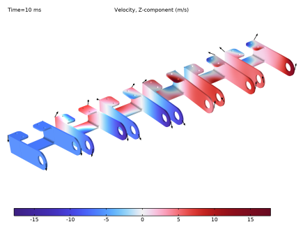
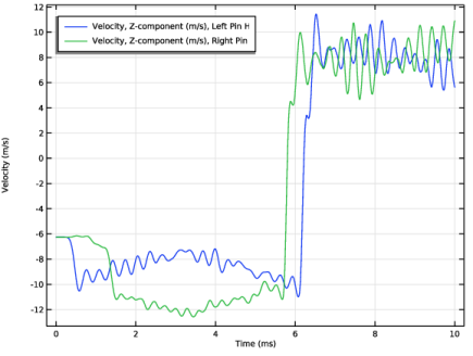
Click Replace Expression in the upper-right corner of the Expression section. From the menu, choose Component 1 (comp1) > Solid Mechanics, Explicit Dynamics > Acceleration and velocity > Velocity - m/s > solid.u_tZ - Velocity, Z-component.
Right Pin Hole
1
Right-click Left Pin Hole and choose Duplicate.
2
In the Settings window for Point Probe, type Right Pin Hole in the Label text field.
3
Study 1
Step 1: Explicit Dynamics
1
In the Model Builder window, under Study 1 click Step 1: Explicit Dynamics.
2
In the Settings window for Explicit Dynamics, locate the Results While Solving section.
3
From the Update at list, choose Time steps taken by solver.
4
In the Study toolbar, click  Compute.
Results
Probe Plot Group 3
1
In the Model Builder window, under Results click Probe Plot Group 3.
2
In the Settings window for 1D Plot Group, locate the Plot Settings section.
3
Select the y-axis label checkbox. In the associated text field, type Velocity (m/s).
4
Locate the Legend section. From the Position list, choose Upper left.
Add an array plot to visualize the impact of the bracket at different times.
Velocity
1
In the Results toolbar, click  3D Plot Group.
2
In the Settings window for 3D Plot Group, type Velocity in the Label text field.
3
Click to expand the Selection section. From the Geometric entity level list, choose Domain.
4
5
Locate the Plot Settings section. Clear the Plot dataset edges checkbox.
Surface 1
1
Right-click Velocity and choose Surface.
2
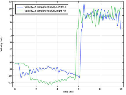
In the Settings window for Surface, click Replace Expression in the upper-right corner of the Expression section. From the menu, choose Component 1 (comp1) > Solid Mechanics, Explicit Dynamics > Acceleration and velocity > Velocity - m/s > solid.u_tZ - Velocity, Z-component.
3
Locate the Coloring and Style section. From the Color table list, choose Wave.
4
From the Scale list, choose Linear symmetric.
Deformation 1
1
Right-click Surface 1 and choose Deformation.
2
In the Settings window for Deformation, locate the Scale section.
3
Select the Scale factor checkbox. In the associated text field, type 1.
Solution Array 1
1
In the Model Builder window, right-click Surface 1 and choose Solution Array.
2
In the Settings window for Solution Array, locate the Data section.
3
From the Time selection list, choose Manual.
4
In the Time indices (1-51) text field, type range(1,10,51).
Velocity
In the Model Builder window, under Results click Velocity.
Arrow Point 1
1
In the Velocity toolbar, click  More Plots and choose Arrow Point.
2
In the Settings window for Arrow Point, click Replace Expression in the upper-right corner of the Expression section. From the menu, choose Component 1 (comp1) > Solid Mechanics, Explicit Dynamics > Acceleration and velocity > solid.u_tX,solid.u_tY,solid.u_tZ - Velocity.
3
Click to expand the Title section. From the Title type list, choose None.
4
Locate the Coloring and Style section. From the Arrow length list, choose Normalized.
5
Select the Scale factor checkbox. In the associated text field, type 0.003.
6
From the Color list, choose Black.
7
Click to expand the Plot Array section. Select the Manual indexing checkbox.
8
Click to expand the Inherit Style section. From the Plot list, choose Surface 1.
Deformation 1
Right-click Arrow Point 1 and choose Deformation.
Solution Array 1
1
In the Model Builder window, right-click Arrow Point 1 and choose Solution Array.
2
In the Settings window for Solution Array, locate the Data section.
3
From the Time selection list, choose Manual.
4
In the Time indices (1-51) text field, type range(1,10,51).
Selection 1
1
Right-click Arrow Point 1 and choose Selection.
2
Velocity
1
In the Model Builder window, under Results click Velocity.
2
In the Settings window for 3D Plot Group, locate the Color Legend section.
3
From the Position list, choose Bottom.
4
In the Velocity toolbar, click  Plot.
5
Click the  Zoom Extents button in the Graphics toolbar.
Add a plot showing the most important energy contributions to verify that the solution is sound.
Energy Balance
1
In the Results toolbar, click  1D Plot Group.
2
In the Settings window for 1D Plot Group, type Energy Balance in the Label text field.
3
Locate the Plot Settings section.
4
Select the y-axis label checkbox. In the associated text field, type Energy (J).
Global 1
1
Right-click Energy Balance and choose Global.
2
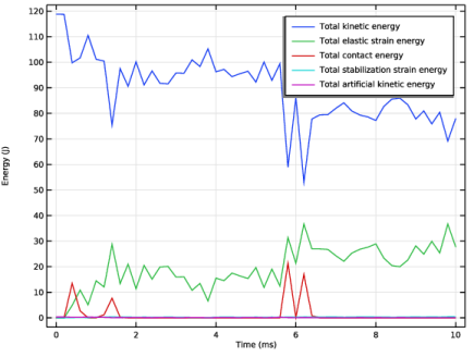
In the Settings window for Global, click Replace Expression in the upper-right corner of the y-Axis Data section. From the menu, choose Component 1 (comp1) > Solid Mechanics, Explicit Dynamics > Global > solid.Wk_tot - Total kinetic energy - J.
3
Click Add Expression in the upper-right corner of the y-Axis Data section. From the menu, choose Component 1 (comp1) > Solid Mechanics, Explicit Dynamics > Global > solid.Ws_tot - Total elastic strain energy - J.
4
Click Add Expression in the upper-right corner of the y-Axis Data section. From the menu, choose Component 1 (comp1) > Solid Mechanics, Explicit Dynamics > Global > solid.Wcnt_tot - Total contact energy - J.
5
Click Add Expression in the upper-right corner of the y-Axis Data section. From the menu, choose Component 1 (comp1) > Solid Mechanics, Explicit Dynamics > Global > solid.Wstb_tot - Total stabilization strain energy - J.
6
Click Add Expression in the upper-right corner of the y-Axis Data section. From the menu, choose Component 1 (comp1) > Solid Mechanics, Explicit Dynamics > Global > solid.Wka_tot - Total artificial kinetic energy - J.
7
In the Energy Balance toolbar, click  Plot.
Evaluate the maximum stress in the bracket during the event.
Evaluation Group 2
In the Results toolbar, click  Evaluation Group.
Volume Maximum 1
1
Right-click Evaluation Group 2 and choose Maximum > Volume Maximum.
2
Click the  Select All button in the Graphics toolbar.
3
4
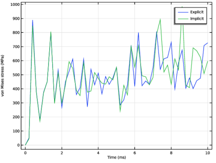
In the Settings window for Volume Maximum, click Replace Expression in the upper-right corner of the Expressions section. From the menu, choose Component 1 (comp1) > Solid Mechanics, Explicit Dynamics > Stress > solid.misesGp - von Mises stress - N/m².
5
In the Evaluation Group 2 toolbar, click  Evaluate.
Evaluation Group 2
1
Go to the Evaluation Group 2 window.
2
Click the Table Graph button in the window toolbar.
Results
Stress History
1
In the Model Builder window, under Results click 1D Plot Group 6.
2
In the Settings window for 1D Plot Group, type Stress History in the Label text field.
The Solid Mechanics, Explicit Dynamics physics interface can be used also with implicit solvers. Hence, to compare the explicit dynamics solution to an implicit dynamics solution, you only need to add a new study with a Time Dependent step that will generate a default solver with an implicit time-dependent solver type.
Add Study
1
In the Home toolbar, click  Windows and choose Add Study.
2
Go to the Add Study window.
3
Find the Studies subsection. In the Select Study tree, select General Studies > Time Dependent.
4
Click the Add Study button in the window toolbar.
Study 2
Step 1: Time Dependent
1
In the Settings window for Time Dependent, locate the Study Settings section.
2
From the Time unit list, choose ms.
3
In the Output times text field, type range(0,0.2,10).
The explicit Verlet solver has zero algorithmic damping. Use a stricter relative tolerance to force smaller time steps in order to reduce the amount of damping of the implicit solver.
4
From the Tolerance list, choose User controlled.
5
In the Relative tolerance text field, type 0.0001.
Duplicate the existing probes to store the probe output from both studies in the model.
Definitions
Left Pin Hole (point1), Right Pin Hole (point2)
1
In the Model Builder window, under Component 1 (comp1) > Definitions, Ctrl-click to select Left Pin Hole (point1) and Right Pin Hole (point2).
2
Left Pin Hole 1 (point3), Right Pin Hole 1 (point4)
1
In the Settings window for Point Probe, click to expand the Table and Window Settings section.
2
Click  Add Table.
3
Click  Add Plot Window.
Right Pin Hole 1 (point4)
1
In the Model Builder window, click Right Pin Hole 1 (point4).
2
In the Settings window for Point Probe, locate the Table and Window Settings section.
3
From the Output table list, choose Table 2.
4
From the Plot window list, choose Probe Plot 2.
Study 2
Step 1: Time Dependent
1
In the Model Builder window, under Study 2 click Step 1: Time Dependent.
2
In the Settings window for Time Dependent, click to expand the Results While Solving section.
3
From the Probes list, choose Manual.
4
In the Probes list, choose Left Pin Hole (point1) and Right Pin Hole (point2).
5
Under Probes, click  Delete.
6
In the Study toolbar, click  Compute.
Results
Probe Plot, Implicit
1
In the Model Builder window, under Results click Probe Plot Group 7.
2
In the Settings window for 1D Plot Group, type Probe Plot, Implicit in the Label text field.
3
Locate the Plot Settings section.
4
Select the y-axis label checkbox. In the associated text field, type Velocity (m/s).
5
Locate the Legend section. From the Position list, choose Upper left.
Extend some existing plots to compare the results of the implicit solution with the explicit solution.
Volume Maximum 2
1
In the Model Builder window, under Results > Evaluation Group 2 right-click Volume Maximum 1 and choose Duplicate.
2
In the Settings window for Volume Maximum, locate the Data section.
3
From the Dataset list, choose Probe Solution 2 (sol2).
4
In the Evaluation Group 2 toolbar, click  Evaluate.
Stress History
1
In the Model Builder window, under Results click Stress History.
2
In the Settings window for 1D Plot Group, locate the Plot Settings section.
3
Select the y-axis label checkbox. In the associated text field, type von Mises stress (MPa).
Table Graph 1
1
In the Model Builder window, click Table Graph 1.
2
In the Settings window for Table Graph, click to expand the Legends section.
3
Select the Show legends checkbox.
4
From the Legends list, choose Manual.
5
6
In the Stress History toolbar, click  Plot.
If you want to generate a model which is identical to the one in the Application Libraries, follow the instructions below. Otherwise, the modeling is complete.
Stress, Implicit
1
In the Model Builder window, under Results click Stress (solid) 1.
2
In the Settings window for 3D Plot Group, type Stress, Implicit in the Label text field.
Probe Plot, Implicit
1
In the Model Builder window, click Probe Plot, Implicit.
2
Drag and drop below Stress, Implicit.
Probe Plot
1
In the Model Builder window, under Results click Probe Plot Group 3.
2
In the Settings window for 1D Plot Group, type Probe Plot, Explicit in the Label text field.
3
In the Label text field, type Probe Plot.
Study 1
Step 1: Explicit Dynamics
1
In the Model Builder window, under Study 1 click Step 1: Explicit Dynamics.
2
In the Settings window for Explicit Dynamics, locate the Results While Solving section.
3
From the Probes list, choose Manual.
4
In the Probes list, choose Left Pin Hole 1 (point3) and Right Pin Hole 1 (point4).
5
Under Probes, click  Delete.
Definitions
Left Pin Hole (point1), Right Pin Hole (point2)
1
In the Model Builder window, under Component 1 (comp1) > Definitions, Ctrl-click to select Left Pin Hole (point1) and Right Pin Hole (point2).
2
Probes, Study 1
In the Settings window for Group, type Probes, Study 1 in the Label text field.
Left Pin Hole 1 (point3), Right Pin Hole 1 (point4)
1
In the Model Builder window, under Component 1 (comp1) > Definitions, Ctrl-click to select Left Pin Hole 1 (point3) and Right Pin Hole 1 (point4).
2
Probes, Study 2
In the Settings window for Group, type Probes, Study 2 in the Label text field.