
|
|
|
|
|
In the Structural Mechanics Modeling chapter of the Structural Mechanics Module User’s Guide: Contact Modeling.
|
|
1
|
|
2
|
In the Application Libraries window, select Structural Mechanics Module > Tutorials > bracket_basic in the tree.
|
|
3
|
Click
|
|
1
|
|
2
|
|
3
|
Click
|
|
4
|
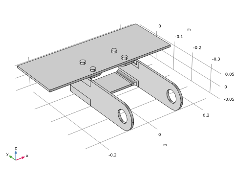
Browse to the model’s Application Libraries folder and double-click the file bracket_bolt_and_support.mphbin.
|
|
5
|
Click
|
|
1
|
|
2
|
|
3
|
|
4
|
Select the object imp2(2) only.
|
|
1
|
|
2
|
|
3
|
|
4
|
|
5
|
|
6
|
|
7
|
Click
|
|
8
|
|
1
|
|
2
|
Go to the Add Material window.
|
|
3
|
|
4
|
Click the Add to Component button in the window toolbar.
|
|
5
|
|
1
|
|
2
|
|
1
|
|
2
|
|
3
|
|
4
|
|
1
|
|
1
|
|
1
|
|
1
|
|
1
|
In the Model Builder window, under Component 1 (comp1) > Solid Mechanics (solid) click Fixed Constraint 1.
|
|
1
|
|
2
|
|
3
|
|
4
|
|
5
|
Click to expand the Contact Surface Offset and Adjustment section. Select the Force zero initial gap checkbox.
|
|
1
|
In the Model Builder window, expand the Component 1 (comp1) > Definitions node, then click Contact Pair 1 (ap1).
|
|
2
|
|
3
|
|
1
|
|
2
|
|
3
|
|
1
|
|
2
|
|
3
|
|
1
|
|
2
|
|
3
|
|
1
|
In the Model Builder window, under Component 1 (comp1) > Solid Mechanics (solid) > Contact 1 click Friction 1.
|
|
2
|
|
3
|
|
4
|
|
1
|
In the Model Builder window, under Component 1 (comp1) > Solid Mechanics (solid) right-click Contact 1 and choose Duplicate.
|
|
2
|
|
3
|
|
4
|
Click
|
|
5
|
|
6
|
Click OK.
|
|
1
|
|
2
|
|
3
|
|
1
|
|
2
|
|
3
|
|
5
|
Select the Group by continuous tangent checkbox.
|
|
1
|
|
2
|
|
3
|
|
1
|
|
2
|
|
3
|
|
4
|
|
1
|
|
2
|
Drag and drop below Edge 1.
|
|
3
|
|
1
|
|
1
|
|
2
|
|
3
|
Click the Custom button.
|
|
4
|
Locate the Element Size Parameters section.
|
|
5
|
|
1
|
|
2
|
Drag and drop below Edge 2.
|
|
3
|
|
1
|
|
2
|
|
3
|
Click to select the
|
|
5
|
Click to expand the Source Faces section. Select Boundaries 3, 23, 55, 59, 72, and 94 only.
|
|
1
|
|
3
|
|
4
|
Click
|
|
6
|
|
7
|
Locate the Element Size Parameters section.
|
|
8
|
|
9
|
Click
|
|
1
|
|
2
|
Go to the Add Study window.
|
|
3
|
Find the Studies subsection. In the Select Study tree, select Preset Studies for Selected Physics Interfaces > Bolt Pretension.
|
|
4
|
Click the Add Study button in the window toolbar.
|
|
5
|
|
1
|
|
2
|
|
3
|
|
1
|
|
2
|
In the Model Builder window, expand the Study 1 > Solver Configurations > Solution 1 (sol1) > Dependent Variables 1 node, then click Displacement Field (comp1.u).
|
|
3
|
|
4
|
|
5
|
|
1
|
|
2
|
|
1
|
|
2
|
|
3
|
|
4
|
|
1
|
|
2
|
|
1
|
|
2
|
Go to the Result Templates window.
|
|
3
|
|
4
|
Click the Add Result Template button in the window toolbar.
|
|
5
|
|
1
|
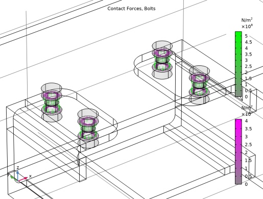
In the Model Builder window, expand the Results > Contact Forces (solid) node, then click Contact Forces (solid).
|
|
2
|
|
1
|
In the Model Builder window, under Results > Contact Forces, Bolts, Ctrl-click to select Contact 1, Pressure and Contact 1, Friction Force.
|
|
2
|
Right-click and choose Disable.
|
|
1
|
|
2
|
|
3
|
|
4
|
|
1
|
|
2
|
|
3
|
|
4
|
|
1
|
|
2
|
|
3
|
|
4
|
Click
|
|
5
|
|
6
|
|
1
|
|
2
|
|
1
|
|
2
|
|
3
|
|
4
|
|
1
|
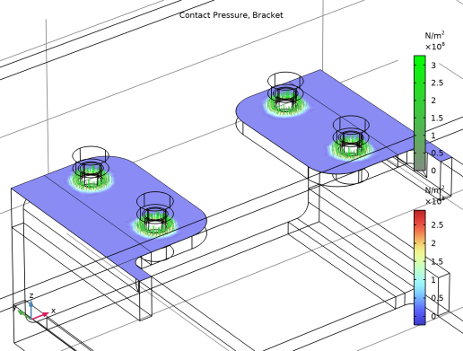
In the Model Builder window, under Results > Contact Pressure, Bracket, Ctrl-click to select Contact 2, Pressure and Contact 2, Friction Force.
|
|
2
|
Right-click and choose Disable.
|
|
1
|
|
2
|
|
3
|
|
4
|
|
5
|
|
1
|
|
2
|
|
1
|
|
2
|
|
3
|
Click to select the
|
|
5
|
Click
|
|
6
|
|
7
|
|
1
|
In the Model Builder window, under Component 1 (comp1) > Solid Mechanics (solid), Ctrl-click to select Contact 1 and Contact 2.
|
|
2
|
Right-click and choose Duplicate.
|
|
1
|
|
2
|
|
3
|
Click
|
|
4
|
|
5
|
Click OK.
|
|
6
|
|
7
|
From the list, choose Augmented Lagrangian.
|
|
8
|
|
1
|
|
2
|
|
3
|
From the list, choose Augmented Lagrangian.
|
|
4
|
|
1
|
|
2
|
|
1
|
|
2
|
|
3
|
|
4
|
|
5
|
Locate the Units section. In the table, enter the following settings:
|
|
6
|
|
1
|
|
2
|
|
3
|
|
4
|
|
1
|
|
2
|
|
3
|
|
4
|
Locate the Coordinate System Selection section. From the Coordinate system list, choose Boundary System 1 (sys1).
|
|
5
|
|
1
|
|
2
|
Go to the Add Study window.
|
|
3
|
|
4
|
Click the Add Study button in the window toolbar.
|
|
5
|
|
1
|
|
2
|
Select the Auxiliary sweep checkbox.
|
|
3
|
Click
|
|
5
|
Click to expand the Values of Dependent Variables section. Find the Initial values of variables solved for subsection. From the Settings list, choose User controlled.
|
|
6
|
|
7
|
|
8
|
Find the Values of variables not solved for subsection. From the Settings list, choose User controlled.
|
|
9
|
|
10
|
|
1
|
|
2
|
|
3
|
In the Model Builder window, expand the Study 2 > Solver Configurations > Solution 2 (sol2) > Dependent Variables 1 node, then click Contact Pressure (comp1.solid.Tn_ap1).
|
|
4
|
|
5
|
|
6
|
In the Model Builder window, under Study 2 > Solver Configurations > Solution 2 (sol2) > Dependent Variables 1 click Contact Pressure (comp1.solid.Tn_ap2).
|
|
7
|
|
8
|
|
9
|
In the Model Builder window, under Study 2 > Solver Configurations > Solution 2 (sol2) > Dependent Variables 1 click Contact Pressure (comp1.solid.Tn_ap3).
|
|
10
|
|
11
|
|
12
|
In the Model Builder window, under Study 2 > Solver Configurations > Solution 2 (sol2) > Dependent Variables 1 click Friction Force (Spatial Frame) (comp1.solid.Tt_ap1).
|
|
13
|
|
14
|
|
15
|
In the Model Builder window, under Study 2 > Solver Configurations > Solution 2 (sol2) > Dependent Variables 1 click Friction Force (Spatial Frame) (comp1.solid.Tt_ap2).
|
|
16
|
|
17
|
|
18
|
In the Model Builder window, under Study 2 > Solver Configurations > Solution 2 (sol2) > Dependent Variables 1 click Friction Force (Spatial Frame) (comp1.solid.Tt_ap3).
|
|
19
|
|
20
|
|
21
|
|
1
|
|
2
|
|
3
|
|
4
|
|
1
|
|
2
|
|
3
|
|
4
|
|
5
|
|
6
|
|
1
|
|
2
|
Go to the Result Templates window.
|
|
3
|
|
4
|
Click the Add Result Template button in the window toolbar.
|
|
5
|
|
1
|
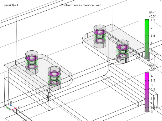
In the Model Builder window, expand the Contact Forces, Service Load node, then click Contact 3, Pressure.
|
|
2
|
|
3
|
|
1
|
|
2
|
|
3
|
|
1
|
In the Model Builder window, expand the Results > Contact Forces, Service Load > Gray Surfaces node, then click Selection 1.
|
|
2
|
|
3
|
|
4
|
Click
|
|
5
|
|
1
|
|
2
|
|
3
|
Select the Modify model configuration for study step checkbox.
|
|
4
|
In the tree, select Component 1 (comp1) > Solid Mechanics (solid), Controls spatial frame > Contact 3.
|
|
5
|
Click
|
|
6
|
In the tree, select Component 1 (comp1) > Solid Mechanics (solid), Controls spatial frame > Contact 4.
|
|
7
|
Click
|
|
8
|
In the tree, select Component 1 (comp1) > Solid Mechanics (solid), Controls spatial frame > Boundary Load 1.
|
|
9
|
Click
|