|
|
|
|
•
|
|
-
|
|
-
|
dynamic viscosity = 0.005 Pa·s
|
|
•
|
|
-
|
|
-
|
Linear elastic behavior: the Lamé parameter μ equals 6.20·106 N/m2, while the other Lamé parameter λ equals 20μ.
|
|
-
|
|
-
|
Linear elastic behavior: the Lamé parameter μ equals 7.20·106 N/m2, while the other Lamé parameter λ equals 20μ.
|
|
•
|
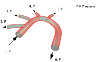
Section 1: 126.09 mmHg
|
|
•
|
Section 2: 125.91 mmHg
|
|
•
|
Section 3: 125.415 mmHg
|
|
•
|
Section 4: 125.415 mmHg
|
|
•
|
Section 5: 125.415 mmHg
|
|
•
|
Section 6: 125.1 mmHg
|

|
1
|
|
2
|
In the Select Physics tree, select Fluid Flow > Fluid–Structure Interaction > Fluid–Solid Interaction, Fixed Geometry.
|
|
3
|
Click Add.
|
|
4
|
Click
|
|
5
|
|
6
|
Click
|
|
1
|
|
2
|
|
1
|
|
2
|
|
3
|
|
4
|
Find the Intervals subsection. In the table, enter the following settings:
|
|
5
|
|
6
|
|
7
|
Click
|
|
1
|
|
2
|
|
3
|
Click
|
|
4
|
Browse to the model’s Application Libraries folder and double-click the file blood_vessel.mphbin.
|
|
5
|
Click
|
|
1
|
|
2
|
|
3
|
|
4
|
Select the object imp1 only.
|
|
5
|
|
1
|
Go to the Cleanup Wizard window.
|
|
2
|
Click Build and Analyze.
|
|
3
|
Click the Apply button in the window toolbar.
|
|
4
|
Click the Apply button in the window toolbar.
|
|
5
|
Click the Done button in the window toolbar.
|
|
6
|
|
1
|
|
2
|
|
3
|
|
1
|
|
2
|
|
1
|
|
2
|
|
3
|
|
5
|
Select the Group by continuous tangent checkbox. The selection should now contain boundaries 10–11, 16–17, 20–21, 23–24, 36–37, 39–40, 42–43, 45–46, 50–53, 58–59, 61–62, 68–69, 71–72, 77–78, 80–81.
|
|
1
|
|
2
|
|
3
|
|
1
|
|
2
|
|
3
|
|
4
|
|
5
|
|
1
|
|
2
|
|
3
|
|
4
|
|
1
|
|
1
|
In the Model Builder window, under Component 1 (comp1) > Solid Mechanics (solid) click Linear Elastic Material 1.
|
|
2
|
|
3
|
|
4
|
|
1
|
|
2
|
|
3
|
|
1
|
In the Model Builder window, under Component 1 (comp1) > Multiphysics click Fluid–Structure Interaction 1 (fsi1).
|
|
2
|
|
3
|
From the Fixed geometry coupling type list, choose Fluid loading on structure to ensure a unidirectional coupling, from the fluid to the solid.
|
|
1
|
In the Model Builder window, under Component 1 (comp1) right-click Materials and choose Blank Material.
|
|
2
|
|
3
|
|
4
|
Locate the Material Contents section. In the table, enter the following settings:
|
|
1
|
|
2
|
|
3
|
|
4
|
Locate the Material Contents section. In the table, enter the following settings:
|
|
1
|
|
2
|
|
3
|
|
4
|
Locate the Material Contents section. In the table, enter the following settings:
|
|
1
|
|
2
|
|
3
|
|
4
|
|
1
|
|
2
|
|
3
|
|
4
|
Locate the Physics and Variables Selection section. In the Solve for column of the table, under Component 1 (comp1), clear the checkbox for Solid Mechanics (solid).
|
|
1
|
|
2
|
|
3
|
In the Solve for column of the table, under Component 1 (comp1), clear the checkbox for Laminar Flow (spf).
|
|
4
|
|
5
|
Click
|
|
7
|
Click to expand the Values of Dependent Variables section. Find the Values of variables not solved for subsection. From the Settings list, choose User controlled.
|
|
8
|
|
9
|
|
10
|
|
1
|
|
2
|
|
3
|
|
4
|
From the Steps taken by solver list, choose Intermediate. This way the solver computes at least once between each output time step in order to reduce possible interpolation errors in the fluid-load evaluation.
|
|
5
|
|
1
|
|
2
|
|
3
|
|
4
|
|
1
|
|
2
|
|
3
|
|
4
|
|
5
|
|
6
|
|
1
|
|
2
|
|
3
|
|
4
|
|
1
|
|
2
|
|
3
|
|
4
|
|
5
|
|
1
|
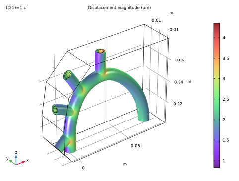
In the Model Builder window, expand the Results > Stress (solid) > Volume 1 node, then click Deformation.
|
|
2
|
|
3
|
|
1
|
|
2
|
Go to the Result Templates window.
|
|
3
|
|
4
|
Click the Add Result Template button in the window toolbar.
|
|
5
|
|
1
|
|
2
|
|
3
|
|
4
|
|
1
|
|
2
|
|
3
|
|
1
|
|
2
|
|
3
|
|
4
|
|
5
|