|
|
|


|
1
|
|
2
|
|
3
|
Click Add.
|
|
4
|
Click
|
|
5
|
|
6
|
Click
|
|
1
|
|
2
|
|
1
|
|
2
|
|
3
|
|
1
|
|
2
|
|
3
|
|
4
|
|
5
|
|
1
|
|
2
|
|
3
|
|
4
|
|
5
|
|
6
|
|
1
|
|
2
|
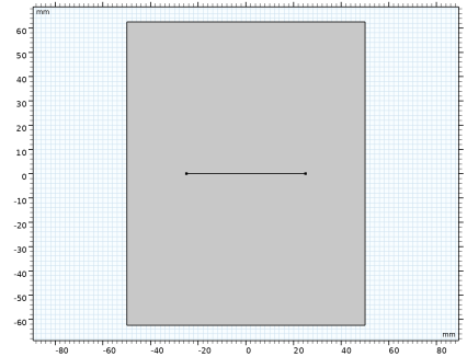
Select the object ls1 only.
|
|
3
|
|
4
|
|
5
|
|
1
|
In the Model Builder window, under Component 1 (comp1) right-click Materials and choose Blank Material.
|
|
2
|
|
1
|
|
1
|
|
1
|
|
1
|
|
3
|
|
4
|
|
1
|
|
3
|
|
4
|
|
1
|
|
2
|
|
3
|
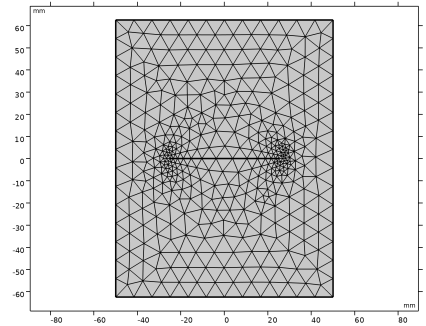
From the list, choose User-controlled mesh.
|
|
1
|
|
2
|
|
3
|
Click the Custom button.
|
|
4
|
Locate the Element Size Parameters section.
|
|
5
|
|
6
|
|
1
|
|
2
|
|
3
|
Click
|
|
5
|
|
1
|
|
2
|
|
3
|
Click
|
|
4
|
|
5
|
Click OK.
|
|
6
|
|
8
|
Click
|
|
9
|
|
10
|
Click OK.
|
|
11
|
|
13
|
Click
|
|
1
|
|
2
|
|
3
|
|
4
|
|
5
|
|
6
|
|
7
|
|
8
|
Clear the Color checkbox.
|
|
9
|
Clear the Color and data range checkbox.
|
|
10
|
Clear the Height scale factor checkbox.
|
|
11
|
Clear the Tube radius scale factor checkbox.
|
|
1
|
|
3
|
|
1
|
|
2
|
|
3
|
Clear the Plot dataset edges checkbox.
|
|
4
|
|
5
|
Click
|
|
6
|
Click
|
|
1
|
|
2
|
Go to the Result Templates window.
|
|
3
|
|
4
|
Click the Add Result Template button in the window toolbar.
|
|
5
|
In the tree, select Study 1/Parametric Solutions 1 (sol2) > Solid Mechanics > Fracture Mechanics Results (solid).
|
|
6
|
Click the Add Result Template button in the window toolbar.
|
|
7
|
|
1
|
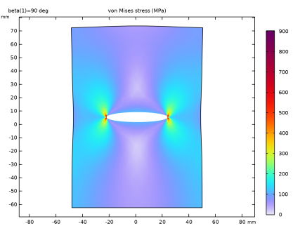
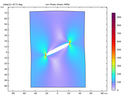
In the Model Builder window, expand the Results > Cracks (solid) node, then click Crack Growth Direction (Crack 1).
|
|
2
|
|
3
|
Clear the Scale factor checkbox.
|
|
1
|
|
2
|
In the Settings window for 2D Plot Group, click
|
|
3
|
Click
|
|
1
|
In the Model Builder window, expand the Results > Fracture Mechanics Results (solid) node, then click Stress Intensity Factors, Mode 1.
|
|
2
|
|
1
|
|
2
|
|
4
|
|
1
|
|
2
|
|
3
|
|
4
|
|
5
|
|
1
|
|
2
|
|
1
|
|
2
|
Select the Manual indexing checkbox.
|
|
1
|
|
2
|
|
1
|
|
2
|
|
3
|
|
1
|
|
3
|
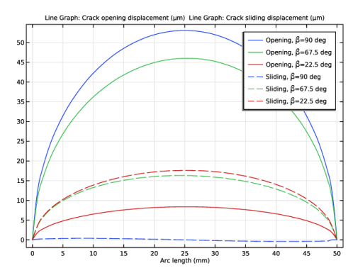
In the Settings window for Line Graph, click Replace Expression in the upper-right corner of the y-Axis Data section. From the menu, choose Component 1 (comp1) > Solid Mechanics > Cracks > Crack displacement - m > solid.crack1.jint1.delta_u1 - Crack opening displacement.
|
|
4
|
|
5
|
|
1
|
|
3
|
In the Settings window for Line Graph, click Replace Expression in the upper-right corner of the y-Axis Data section. From the menu, choose Component 1 (comp1) > Solid Mechanics > Cracks > Crack displacement - m > solid.crack1.jint1.delta_u2 - Crack sliding displacement.
|
|
4
|
Click to expand the Coloring and Style section. Find the Line style subsection. From the Line list, choose Dashed.
|
|
5
|
|
6
|
|
7
|
|
8
|