PDF

Solving the Hydrogen Atom
Introduction
In this tutorial model, we take a look at perhaps the most significant exact results of quantum mechanics — the ground state and the first few excited states of the hydrogen atom — and go over how to reproduce these results using COMSOL Multiphysics.
The hydrogen atom with its single electron is described by the time-independent Schrödinger equation (TISE):
(1)
Here, , m, e, and ε0 are the reduced Planck constant, electron mass, elementary charge, and the permittivity of vacuum, respectively. The dependent variable to be solved for, ψ(r), is the wave function: a complex scalar field whose norm, | ψ(r) |2, gives the probability of finding the electron at r. The operator , is the Hamiltonian, which corresponds to the total energy of the system. The Laplacian term gives the kinetic energy of the electron, whereas the potential energy is simply given by the Coulomb potential due to the positively charged nucleus at the origin. The TISE is in the form of an eigenvalue problem for the unknown total energy, E, and can be solved exactly by the usual tools of the trade: separation of variables and series expansions. The resulting eigenstates are labeled by three integers: the quantum numbers, n, l, and m, where n, l ∈ N, l ≤ n and m = −l, …, 0, …, l. Using spherical polar coordinates with θ and ϕ denoting the polar and azimuthal angles, respectively, they can be expressed as
(2)
where Rnl(r) is the radial wave functions and , expressed in terms of the Legendre polynomials , are known as the spherical harmonics. The eigenenergy only depends on the principal quantum number, n:
(3)
where RH ≈ 13.6057 eV is known as the Rydberg constant.
Model Definition
In the case of the hydrogen atom, the TISE is simply a PDE for a complex-valued scalar field in 3D, thus allowing for a FEM-based solution of the eigenvalue problem. The Semiconductor Module, an add-on to COMSOL Multiphysics, offers a Schrödinger Equation interface (abbreviated as schr), which we can use for building our hydrogen atom model.
Set up a sphere of radius A0 = 15a0, where a0 = 2/(mee2) ≈ 52.9 pm is the Bohr radius. In the Schrödinger Equation interface, modify the default nodes (Effective Mass and Electron Potential Energy) so that the effective mass is equal to me (this model does not use a periodic lattice) and the electron potential energy is equal to the Coulomb potential of the nucleus. The only boundary condition needed here is ψ → 0 as r → ∞, which corresponds to bound states. Therefore, surround the sphere with a thin layer and define it as an infinite element domain. To improve the computation speed, use a mesh that becomes progressively coarser in the radial direction. Finally, specify the energy scale as eV and estimate 15 eV as the starting point for the eigenvalue search.
Results and Discussion
Table 1 shows the eigenenergies obtained for the first two principal quantum numbers together with their theoretical values.
(RH/n2 (eV))
(En (eV) from schr)
Note that the eigenvalues depend on the mesh used, so we always recommend running a mesh refinement study to get reliable results. Figure 1 shows the shape of the eigenstates, or orbitals, plotted using 3D isosurface plots.
Figure 1: Orbital shapes of unperturbed hydrogen, visualized using a series of displaced 3D isosurface plots.
Adopt the labeling used extensively in atomic physics: 1s, 2s, 2px, …. It is clear from the figure that the s-states are radially symmetric, whereas each of the p-states has cylindrical symmetry along one of three mutually perpendicular axes. For the spherically symmetric s-states, the radial probability density has the simple analytical form
(4)
Figure 2 and Figure 3 show a comparison between the analytical and simulated results.
Figure 2: Radial probability of the 1s state (ground state). Analytical results are shown using solid lines, while numerical result obtained in COMSOL Multiphysics are shown using point markers.
Figure 3: Radial probability of the 2s state (first excited state). Analytical results are shown using solid lines, while numerical result obtained in COMSOL Multiphysics are shown using point markers.
Stark Effect
In the hydrogen atom, the Stark effect can be observed as a possible shift of the energy levels, when an external electric field is applied.The perturbation can be represented by the Hamiltonian VStark = eεextz. To implement the Stark effect in COMSOL Multiphysics, simply add another Electron Potential Energy node to the model. Then, the split energy levels and the corresponding orbital shapes can readily be obtained. To make the effect clearly visible, use an extremely high external field of ∼ 2×10⁸ V/m.
See the Modeling Instructions section for more detailed explanations on the model setup.
Application Library path: Semiconductor_Module/Quantum_Systems/solving_hydrogen_atom
Modeling Instructions
From the File menu, choose New.
New
In the New window, click  Model Wizard.
Model Wizard
1
In the Model Wizard window, click  3D.
2
In the Select Physics tree, select Semiconductor > Schrödinger Equation (schr).
3
Click Add.
4
Click  Study.
5
In the Select Study tree, select Preset Studies for Selected Physics Interfaces > Eigenvalue.
6
Global Definitions
Parameters 1
1
In the Model Builder window, under Global Definitions click Parameters 1.
2
In the Settings window for Parameters, locate the Parameters section.
3
Click  Load from File.
4
Geometry 1
Sphere 1 (sph1)
1
In the Geometry toolbar, click  Sphere.
2
In the Settings window for Sphere, locate the Size section.
3
In the Radius text field, type A0+0.1*A0.
4
Click to expand the Layers section. In the table, enter the following settings:
Point 1 (pt1)
In the Geometry toolbar, click  More Primitives and choose Point.
Definitions
Variables 1
1
In the Model Builder window, under Component 1 (comp1) right-click Definitions and choose Variables.
2
In the Settings window for Variables, locate the Variables section.
3
Simulation domain
1
In the Definitions toolbar, click  Explicit.
2
In the Settings window for Explicit, type Simulation domain in the Label text field.
3
Infinite element domain
1
In the Definitions toolbar, click  Complement.
2
In the Settings window for Complement, type Infinite element domain in the Label text field.
3
Locate the Input Entities section. Under Selections to invert, click  Add.
4
In the Add dialog, select Simulation domain in the Selections to invert list.
5
Exterior boundary
1
In the Definitions toolbar, click  Adjacent.
2
In the Settings window for Adjacent, type Exterior boundary in the Label text field.
3
Locate the Input Entities section. Under Input selections, click  Add.
4
In the Add dialog, in the Input selections list, choose Simulation domain and Infinite element domain.
5
Interior boundary
1
In the Definitions toolbar, click  Adjacent.
2
In the Settings window for Adjacent, type Interior boundary in the Label text field.
3
Locate the Input Entities section. Under Input selections, click  Add.
4
In the Add dialog, select Simulation domain in the Input selections list.
5
Spherical System 2 (sys2)
In the Definitions toolbar, click  Coordinate Systems and choose Spherical System.
Infinite Element Domain 1 (ie1)
1
In the Definitions toolbar, click  Infinite Element Domain.
2
In the Settings window for Infinite Element Domain, locate the Domain Selection section.
3
From the Selection list, choose Infinite element domain.
4
Locate the Geometry section. From the Type list, choose Spherical.
Schrödinger Equation (schr)
1
In the Model Builder window, under Component 1 (comp1) click Schrödinger Equation (schr).
2
In the Settings window for Schrödinger Equation, locate the Model Properties section.
3
Find the Stationary study subsection. In the E text field, type -15[eV].
Effective Mass 1
1
In the Model Builder window, under Component 1 (comp1) > Schrödinger Equation (schr) click Effective Mass 1.
2
In the Settings window for Effective Mass, locate the Effective Mass section.
3
In the meff,e,11 text field, type me_const.
Nucleus
1
In the Model Builder window, under Component 1 (comp1) > Schrödinger Equation (schr) click Electron Potential Energy 1.
2
In the Settings window for Electron Potential Energy, type Nucleus in the Label text field.
3
Locate the Electron Potential Energy section. From the Ve list, choose User defined. In the associated text field, type -kC*e_const^2/sys2.r.
Zero Probability 1
1
In the Physics toolbar, click  Boundaries and choose Zero Probability.
2
In the Settings window for Zero Probability, locate the Boundary Selection section.
3
From the Selection list, choose Exterior boundary.
External field along z-axis
1
In the Physics toolbar, click  Domains and choose Electron Potential Energy.
2
In the Settings window for Electron Potential Energy, type External field along z-axis in the Label text field.
3
Locate the Domain Selection section. From the Selection list, choose All domains.
4
Locate the Electron Potential Energy section. From the Ve list, choose User defined. In the associated text field, type e_const*Eext*z.
Mesh 1
1
In the Model Builder window, under Component 1 (comp1) click Mesh 1.
2
In the Settings window for Mesh, locate the Sequence Type section.
3
From the list, choose User-controlled mesh.
Size
1
In the Model Builder window, under Component 1 (comp1) > Mesh 1 click Size.
2
In the Settings window for Size, locate the Element Size section.
3
Click the Custom button.
4
Locate the Element Size Parameters section. In the Maximum element size text field, type 10*h0.
5
In the Minimum element size text field, type 0.1*h0.
Free Tetrahedral 1
1
In the Model Builder window, click Free Tetrahedral 1.
2
In the Settings window for Free Tetrahedral, locate the Domain Selection section.
3
From the Geometric entity level list, choose Domain.
4
From the Selection list, choose Simulation domain.
Size Expression 1
1
Right-click Free Tetrahedral 1 and choose Size Expression.
2
In the Settings window for Size Expression, locate the Element Size Expression section.
3
In the Size expression text field, type (1+sqrt(x^2+y^2+z^2)*hg)*h0.
Swept 1
1
In the Mesh toolbar, click  Swept.
2
In the Settings window for Swept, locate the Domain Selection section.
3
From the Geometric entity level list, choose Domain.
4
From the Selection list, choose Infinite element domain.
5
Click to expand the Source Faces section. From the Selection list, choose Interior boundary.
6
Click to expand the Destination Faces section. From the Selection list, choose Exterior boundary.
Distribution 1
Right-click Swept 1 and choose Distribution.
No External Field
In the Settings window for Study, type No External Field in the Label text field.
Step 1: Eigenvalue
1
In the Model Builder window, under No External Field click Step 1: Eigenvalue.
2
In the Settings window for Eigenvalue, locate the Study Settings section.
3
In the Desired number of eigenvalues text field, type 5.
4
In the Search for eigenvalues around shift text field, type -15.
5
Locate the Physics and Variables Selection section. Select the Modify model configuration for study step checkbox.
6
In the tree, select Component 1 (comp1) > Schrödinger Equation (schr) > External field along z-axis.
7
Click  Disable.
8
In the Study toolbar, click  Compute.
Results
Cut Line 3D 1
1
In the Results toolbar, click  Cut Line 3D.
2
In the Settings window for Cut Line 3D, locate the Line Data section.
3
In row Point 2, set X to 0.
4
In row Point 2, set Z to A0.
1s Radial Probability
1
In the Results toolbar, click  1D Plot Group.
2
In the Settings window for 1D Plot Group, type 1s Radial Probability in the Label text field.
3
Locate the Data section. From the Dataset list, choose Cut Line 3D 1.
4
From the Eigenvalue selection list, choose First.
5
Locate the Plot Settings section.
6
Select the x-axis label checkbox. In the associated text field, type r/a<sub>0</sub>.
7
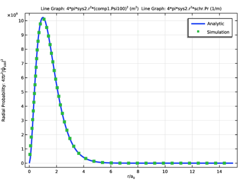
Select the y-axis label checkbox. In the associated text field, type Radial Probability: 4\pi r<sup>2</sup>|\psi<sub>100</sub>|<sup>2</sup>.
Line Graph 1
1
Right-click 1s Radial Probability and choose Line Graph.
2
In the Settings window for Line Graph, locate the y-Axis Data section.
3
In the Expression text field, type 4*pi*sys2.r^2*(comp1.Psi100)^2.
4
Locate the x-Axis Data section. From the Parameter list, choose Expression.
5
In the Expression text field, type sys2.r/a0_const.
6
Click to expand the Coloring and Style section. From the Width list, choose 3.
7
Click to expand the Legends section. Select the Show legends checkbox.
8
From the Legends list, choose Manual.
9
10
Click to expand the Quality section. From the Evaluation settings list, choose Manual.
11
From the Resolution list, choose Finer.
Line Graph 2
1
In the Model Builder window, right-click 1s Radial Probability and choose Line Graph.
2
In the Settings window for Line Graph, locate the y-Axis Data section.
3
In the Expression text field, type 4*pi*sys2.r^2*schr.Pr.
4
Locate the x-Axis Data section. From the Parameter list, choose Expression.
5
In the Expression text field, type sys2.r/a0_const.
6
Locate the Coloring and Style section. Find the Line style subsection. From the Line list, choose None.
7
From the Width list, choose 3.
8
Find the Line markers subsection. From the Marker list, choose Point.
9
From the Positioning list, choose Interpolated.
10
In the Number text field, type 50.
11
Locate the Legends section. Select the Show legends checkbox.
12
From the Legends list, choose Manual.
13
14
In the 1s Radial Probability toolbar, click  Plot.
2s Radial Probability
1
Right-click 1s Radial Probability and choose Duplicate.
2
In the Settings window for 1D Plot Group, type 2s Radial Probability in the Label text field.
3
Locate the Data section. From the Eigenvalue selection list, choose Manual.
4
In the Eigenvalue indices (1-5) text field, type 2.
5
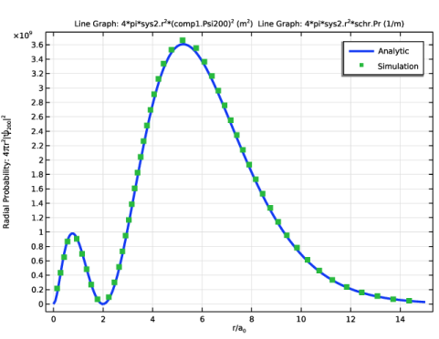
Locate the Plot Settings section. In the y-axis label text field, type Radial Probability: 4\pi r<sup>2</sup>|\psi<sub>200</sub>|<sup>2</sup>.
Line Graph 1
1
In the Model Builder window, expand the 2s Radial Probability node, then click Line Graph 1.
2
In the Settings window for Line Graph, locate the y-Axis Data section.
3
In the Expression text field, type 4*pi*sys2.r^2*(comp1.Psi200)^2.
4
In the 2s Radial Probability toolbar, click  Plot.
Unperturbed orbital shapes
1
In the Results toolbar, click  3D Plot Group.
2
In the Settings window for 3D Plot Group, type Unperturbed orbital shapes in the Label text field.
3
Click to expand the Title section. From the Title type list, choose Manual.
4
In the Title text area, type Unperturbed Orbital Shapes.
5
Locate the Plot Settings section. Clear the Plot dataset edges checkbox.
6
Locate the Color Legend section. Clear the Show legends checkbox.
Isosurface 1
1
Right-click Unperturbed orbital shapes and choose Isosurface.
2
In the Settings window for Isosurface, locate the Expression section.
3
In the Expression text field, type schr.Pr.
Isosurface 2
1
In the Model Builder window, right-click Unperturbed orbital shapes and choose Isosurface.
2
In the Settings window for Isosurface, locate the Data section.
3
From the Dataset list, choose No External Field/Solution 1 (sol1).
4
From the Eigenvalue list, choose -3.4016.
5
Locate the Expression section. In the Expression text field, type schr.Pr.
6
Locate the Levels section. Select the Interactive checkbox.
7
In the Shift text field, type -2.45E28.
Transformation 1
1
Right-click Isosurface 2 and choose Transformation.
2
In the Settings window for Transformation, locate the Transformation section.
3
In the X text field, type 7E-10.
Isosurface 3
1
In the Model Builder window, right-click Unperturbed orbital shapes and choose Isosurface.
2
In the Settings window for Isosurface, locate the Data section.
3
From the Dataset list, choose No External Field/Solution 1 (sol1).
4
From the Eigenvalue list, choose -3.401.
5
Locate the Expression section. In the Expression text field, type schr.Pr.
Transformation 1
1
Right-click Isosurface 3 and choose Transformation.
2
In the Settings window for Transformation, locate the Transformation section.
3
In the X text field, type 15E-10.
Isosurface 4
1
In the Model Builder window, right-click Unperturbed orbital shapes and choose Isosurface.
2
In the Settings window for Isosurface, locate the Data section.
3
From the Dataset list, choose No External Field/Solution 1 (sol1).
4
From the Eigenvalue list, choose -3.401.
5
Locate the Expression section. In the Expression text field, type schr.Pr.
Transformation 1
1
Right-click Isosurface 4 and choose Transformation.
2
In the Settings window for Transformation, locate the Transformation section.
3
In the X text field, type 15E-10.
4
In the Z text field, type 7.5E-10.
Isosurface 5
1
In the Model Builder window, right-click Unperturbed orbital shapes and choose Isosurface.
2
In the Settings window for Isosurface, locate the Data section.
3
From the Dataset list, choose No External Field/Solution 1 (sol1).
4
From the Eigenvalue list, choose -3.401.
5
Locate the Expression section. In the Expression text field, type schr.Pr.
Transformation 1
1
Right-click Isosurface 5 and choose Transformation.
2
In the Settings window for Transformation, locate the Transformation section.
3
In the X text field, type 15E-10.
4
In the Z text field, type -7.5E-10.
Annotation 1
1
In the Model Builder window, right-click Unperturbed orbital shapes and choose Annotation.
2
In the Settings window for Annotation, locate the Annotation section.
3
In the Text text field, type 1s.
4
Locate the Position section. In the Z text field, type 2E-10.
5
Locate the Coloring and Style section. Clear the Show point checkbox.
6
From the Anchor point list, choose Center.
Annotation 2
1
Right-click Unperturbed orbital shapes and choose Annotation.
2
In the Settings window for Annotation, locate the Annotation section.
3
In the Text text field, type 2s.
4
Locate the Position section. In the X text field, type 7E-10.
5
In the Z text field, type 5E-10.
6
Locate the Coloring and Style section. Clear the Show point checkbox.
7
From the Anchor point list, choose Center.
Annotation 3
1
Right-click Unperturbed orbital shapes and choose Annotation.
2
In the Settings window for Annotation, locate the Annotation section.
3
In the Text text field, type 2p.
4
Locate the Position section. In the X text field, type 15E-10.
5
In the Z text field, type 12.5E-10.
6
Locate the Coloring and Style section. Clear the Show point checkbox.
7
From the Anchor point list, choose Center.
8
Click the  Go to XZ View button in the Graphics toolbar.
9
Click the  Transparency button in the Graphics toolbar.
10
In the Unperturbed orbital shapes toolbar, click  Plot.
Add Study
1
In the Home toolbar, click  Add Study to open the Add Study window.
2
Go to the Add Study window.
3
Find the Studies subsection. In the Select Study tree, select Preset Studies for Selected Physics Interfaces > Eigenvalue.
4
Click the Add Study button in the window toolbar.
5
In the Home toolbar, click  Add Study to close the Add Study window.
Stark Effect
In the Settings window for Study, type Stark Effect in the Label text field.
Step 1: Eigenvalue
1
In the Model Builder window, under Stark Effect click Step 1: Eigenvalue.
2
In the Settings window for Eigenvalue, locate the Study Settings section.
3
In the Desired number of eigenvalues text field, type 5.
4
In the Search for eigenvalues around shift text field, type -15.
5
In the Study toolbar, click  Compute.
Results
Stark effect orbital shapes
1
In the Model Builder window, right-click Unperturbed orbital shapes and choose Duplicate.
2
In the Settings window for 3D Plot Group, type Stark effect orbital shapes in the Label text field.
3
Locate the Data section. From the Dataset list, choose Stark Effect/Solution 2 (sol2).
4
Locate the Title section. In the Title text area, type Stark Effect Orbital Shapes.
5
In the Model Builder window, expand the Stark effect orbital shapes node.
Isosurface 2
1
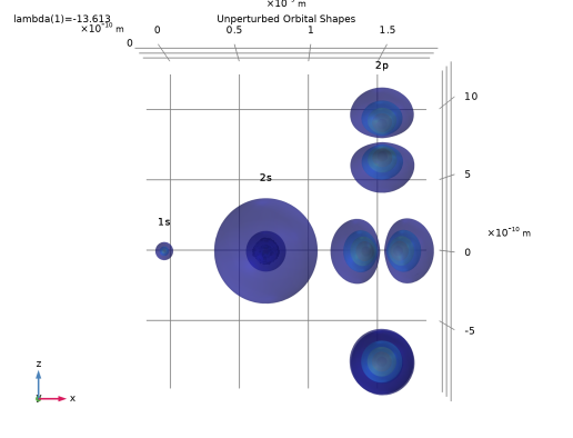
In the Model Builder window, expand the Results > Stark effect orbital shapes > Isosurface 2 node, then click Isosurface 2.
2
In the Settings window for Isosurface, locate the Data section.
3
From the Dataset list, choose Stark Effect/Solution 2 (sol2).
4
From the Eigenvalue list, choose -3.4013.
5
Locate the Levels section. Clear the Interactive checkbox.
Isosurface 3
1
In the Model Builder window, click Isosurface 3.
2
In the Settings window for Isosurface, locate the Data section.
3
From the Dataset list, choose Stark Effect/Solution 2 (sol2).
4
From the Eigenvalue list, choose -3.4013.
Isosurface 4
1
In the Model Builder window, expand the Isosurface 3 node, then click Results > Stark effect orbital shapes > Isosurface 4.
2
In the Settings window for Isosurface, locate the Data section.
3
From the Dataset list, choose Stark Effect/Solution 2 (sol2).
4
From the Eigenvalue list, choose -3.3716.
Transformation 1
1
In the Model Builder window, expand the Isosurface 4 node, then click Transformation 1.
2
In the Settings window for Transformation, locate the Transformation section.
3
In the X text field, type 11E-10.
4
In the Z text field, type 5E-10.
Isosurface 5
1
In the Model Builder window, under Results > Stark effect orbital shapes click Isosurface 5.
2
In the Settings window for Isosurface, locate the Data section.
3
From the Dataset list, choose Stark Effect/Solution 2 (sol2).
4
From the Eigenvalue list, choose -3.4316.
Transformation 1
1
In the Model Builder window, expand the Isosurface 5 node, then click Transformation 1.
2
In the Settings window for Transformation, locate the Transformation section.
3
In the X text field, type 11E-10.
4
In the Z text field, type -5E-10.
Annotation 1
1
In the Model Builder window, under Results > Stark effect orbital shapes click Annotation 1.
2
In the Settings window for Annotation, locate the Annotation section.
3
In the Text text field, type 1s (no splitting).
4
Select the LaTeX markup checkbox.
Annotation 2
1
In the Model Builder window, click Annotation 2.
2
In the Settings window for Annotation, locate the Annotation section.
3
In the Text text field, type 2px, 2py \\ (no splitting).
4
Select the LaTeX markup checkbox.
5
Locate the Position section. In the X text field, type 22E-10.
6
In the Z text field, type 0.
Annotation 3
1
In the Model Builder window, click Annotation 3.
2
In the Settings window for Annotation, locate the Annotation section.
3
In the Text text field, type Hybrid 2s+2pz \\(Stark splitting by +0.03 eV).
4
Select the LaTeX markup checkbox.
5
Locate the Position section. In the X text field, type 11E-10.
6
In the Z text field, type 10E-10.
Annotation 4
1
In the Model Builder window, right-click Stark effect orbital shapes and choose Annotation.
2
In the Settings window for Annotation, locate the Annotation section.
3
In the Text text field, type Hybrid 2s+2pz \\(Stark splitting by -0.03 eV).
4
Select the LaTeX markup checkbox.
5
Locate the Position section. In the X text field, type 11E-10.
6
In the Z text field, type -10E-10.
7
Locate the Coloring and Style section. Clear the Show point checkbox.
8
From the Anchor point list, choose Center.
9
In the Stark effect orbital shapes toolbar, click  Plot.
Unperturbed eigenenergies
1
In the Model Builder window, expand the Results > Derived Values node, then click Eigenvalue.
2
In the Settings window for Global Evaluation, type Unperturbed eigenenergies in the Label text field.
3
Locate the Data section. From the Eigenvalue selection list, choose Manual.
4
In the Eigenvalue indices (1-5) text field, type 1,2.
5
Click  Evaluate.
Stark effect eigenenergies
1
In the Model Builder window, under Results > Derived Values click Eigenvalue 1.
2
In the Settings window for Global Evaluation, type Stark effect eigenenergies in the Label text field.
3
Click  Evaluate.