
|
|
|
|
1
|
|
2
|
|
3
|
Click Add.
|
|
4
|
Click
|
|
5
|
In the Select Study tree, select Preset Studies for Selected Physics Interfaces > Semiconductor Equilibrium.
|
|
6
|
Click
|
|
1
|
|
2
|
|
1
|
|
2
|
|
3
|
|
1
|
|
2
|
|
1
|
|
2
|
Go to the Add Material window.
|
|
3
|
|
4
|
Click the Add to Component button in the window toolbar.
|
|
5
|
|
1
|
|
2
|
|
3
|
Click to expand the Discretization section. From the Formulation list, choose Finite element quasi Fermi level (quadratic shape function).
|
|
1
|
|
3
|
|
4
|
|
5
|
|
6
|
|
1
|
|
2
|
|
3
|
Click
|
|
5
|
|
1
|
In the Model Builder window, under Component 1 (comp1) > Semiconductor (semi) right-click Metal Contact 1 and choose Duplicate.
|
|
2
|
|
3
|
|
1
|
|
2
|
In the Settings window for WKB Tunneling Model, Electrons, locate the Potential Barrier Domain Selection section.
|
|
3
|
Click to select the
|
|
5
|
Locate the Opposite Boundary Selection section. Click to select the
|
|
1
|
|
2
|
|
1
|
|
2
|
In the Settings window for Semiconductor Equilibrium, locate the Physics and Variables Selection section.
|
|
3
|
Select the Modify model configuration for study step checkbox.
|
|
4
|
|
5
|
Click
|
|
1
|
|
2
|
|
3
|
Select the Modify model configuration for study step checkbox.
|
|
4
|
|
5
|
Click
|
|
6
|
|
7
|
Click
|
|
9
|
|
1
|
|
2
|
Go to the Add Study window.
|
|
3
|
|
4
|
Click the Add Study button in the window toolbar.
|
|
5
|
|
1
|
|
2
|
|
3
|
Find the Initial values of variables solved for subsection. From the Settings list, choose User controlled.
|
|
4
|
|
5
|
|
6
|
|
7
|
|
8
|
Click
|
|
10
|
|
1
|
|
2
|
|
3
|
|
4
|
Locate the Plot Settings section.
|
|
5
|
|
6
|
|
7
|
|
1
|
|
2
|
|
3
|
|
4
|
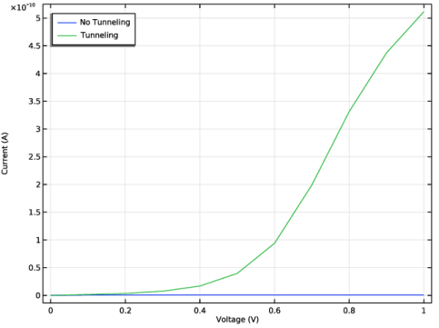
Locate the y-Axis Data section. In the table, enter the following settings:
|
|
5
|
|
6
|
Clear the Solution checkbox.
|
|
7
|
Clear the Description checkbox.
|
|
1
|
|
2
|
|
3
|
|
4
|
Locate the y-Axis Data section. In the table, enter the following settings:
|
|
5
|