
|
|
|
|
1
|
|
2
|
|
3
|
Click Add.
|
|
4
|
Click
|
|
5
|
|
6
|
Click
|
|
1
|
|
2
|
|
1
|
|
2
|
|
3
|
|
1
|
|
2
|
|
3
|
|
4
|
|
5
|
|
1
|
|
2
|
|
3
|
|
4
|
|
5
|
|
1
|
|
2
|
|
3
|
|
4
|
|
1
|
|
2
|
|
3
|
|
4
|
|
5
|
|
6
|
|
1
|
|
2
|
|
3
|
|
4
|
|
5
|
|
6
|
|
1
|
|
2
|
|
3
|
|
4
|
|
1
|
|
2
|
|
3
|
|
4
|
|
5
|
|
1
|
|
2
|
|
3
|
|
1
|
|
2
|
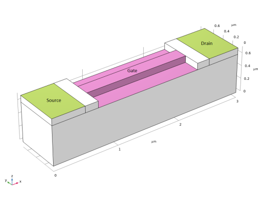
Select the object blk1 only.
|
|
3
|
|
4
|
|
5
|
|
6
|
Click
|
|
1
|
|
2
|
Go to the Add Material window.
|
|
3
|
|
4
|
Click the Add to Component button in the window toolbar.
|
|
5
|
|
1
|
|
2
|
|
3
|
|
4
|
|
1
|
|
2
|
|
3
|
|
4
|
|
5
|
|
6
|
|
7
|
|
8
|
|
9
|
|
10
|
|
11
|
|
12
|
|
1
|
|
2
|
|
3
|
|
1
|
|
2
|
|
1
|
|
2
|
|
3
|
|
5
|
|
1
|
|
2
|
|
3
|
|
5
|
|
1
|
|
3
|
|
4
|
|
5
|
|
6
|
|
1
|
|
2
|
|
3
|
|
1
|
|
1
|
|
2
|
|
3
|
|
1
|
|
2
|
|
3
|
|
1
|
|
2
|
|
3
|
|
4
|
|
1
|
In the Model Builder window, under Component 1 (comp1) > Mesh 1 right-click Swept 1 and choose Duplicate.
|
|
2
|
|
3
|
Click
|
|
1
|
|
2
|
|
3
|
|
4
|
|
5
|
Select the Reverse direction checkbox.
|
|
6
|
Click
|
|
1
|
|
2
|
|
1
|
|
2
|
|
3
|
Select the Auxiliary sweep checkbox.
|
|
4
|
Click
|
|
6
|
Click
|
|
8
|
|
9
|
|
1
|
|
2
|
|
3
|
|
1
|
|
2
|
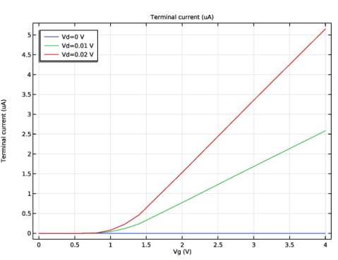
In the Settings window for Global, click Replace Expression in the upper-right corner of the y-Axis Data section. From the menu, choose Component 1 (comp1) > Semiconductor > Terminals > semi.I0_2 - Terminal current - A.
|
|
3
|
Locate the y-Axis Data section. In the table, enter the following settings:
|
|
4
|
|
5
|
|
1
|
|
2
|
Go to the Add Study window.
|
|
3
|
|
4
|
Click the Add Study button in the window toolbar.
|
|
5
|
|
1
|
|
2
|
|
1
|
|
2
|
|
3
|
Find the Initial values of variables solved for subsection. From the Settings list, choose User controlled.
|
|
4
|
|
5
|
|
6
|
|
7
|
|
8
|
|
9
|
Click
|
|
11
|
Click
|
|
13
|
|
14
|
|
15
|
|
1
|
|
2
|
|
3
|
|
4
|