PDF

Electrolyte-Gated Organic Field-Effect Transistor
Introduction
An Electrolyte-Gated Organic Field-Effect Transistor, for short EGOFET, is a type of field-effect transistor where the gate dielectric layer is replaced by an electrolyte and the semiconductor is an organic material. Just like a traditional field-effect transistor, an EGOFET comprises tree electrodes, including source, drain, and gate electrode.
In an EGOFET constructed with a p-type organic semiconductor, the gate is negatively polarized, causing the positive ions of the electrolyte to accumulate at the gate–electrolyte interface. Concurrently, the negative ions accumulate at the electrolyte–organic semiconductor interface. This ends up in the formation of electrical double layer at the two aforementioned interfaces.
In this example, we are going to show how to model the static characteristics of this device based on a general Drift–Diffusion model.
Model Definition
The materials and geometry of this model are a simplified version of the device described in Ref. 1. The model uses the following configuration: source and drain electrodes positioned on the two side ends of the organic semiconductor domain and the gate electrode placed at the top boundary of the electrolyte domain. The total depth of the transistor is 1 cm with a width of 30 μm. Figure 1 shows the configuration of the modeled device.
Figure 1: Configuration of the modeled EGOFET, with the organic semiconductor domain in green and the electrolyte in blue.
In a p-type organic semiconductor, the charge carriers are holes, while in the electrolyte domain, ions serve as the charge carriers. The model uses the Transport of Charge Carriers interface for defining transport phenomena (Equation 1) and the Electrostatics interface to describe the motion of the charges under the applied electric field (Equation 2):
(1)
(2)
In the equations above, Jc, Dc, and zc, are flux, diffusion coefficient, and charge of the charge carriers, respectively. R is the ideal gas constant, T the temperature, F the Faraday constant, and V the electric potential. ε0 and εr are the permittivity of vacuum and relative permittivity of the material, respectively.
Since there are three different types of charge carriers in this device, we use the same set of equations for each, namely the holes, positive ions and negative ions. The procedure of the implementation is described in detail in the Modeling Instructions section.
Results and Discussion
Figure 2 shows the electric field profile at the cross-section of the device (along the y direction) for zero drain voltage and gate voltage varying from 0 to 0.5 V. The profile shows a high electric field at the two interfaces, corresponding to the gate–electrolyte and electrolyte–organic semiconductor interface. This is due to the accumulation of charges at these interfaces.
Figure 2: Electric field along the cross section of the EGOFET.
Figure 3 shows the transfer curve of the EGOFET which is drain current versus the gate voltage.
Figure 3: Drain current versus gate voltage curve.
Reference
1. N. Delavari, K. Tybrandt, M. Berggren, B. Piro, V. Noël, G.Mattana, and I. Zozoulenko, “Nernst–Planck–Poisson analysis of electrolyte-gated organic field-effect transistors,” J. Phys. D: Appl. Phys., vol. 54, no. 41, 415101, 2021.
Application Library path: Semiconductor_Module/Transistors/egofet
Modeling Instructions
From the File menu, choose New.
New
In the New window, click  Model Wizard.
Model Wizard
1
In the Model Wizard window, click  2D.
2
In the Select Physics tree, select Electric Discharge > Transport of Charge Carriers (tcc).
3
Click Add.
4
In the Charge carriers (1/m³) table, enter the following settings:
5
Click Add.
6
In the Number of charge carriers text field, type 2.
7
In the Charge carriers (1/m³) table, enter the following settings:
8
In the Select Physics tree, select AC/DC > Electric Fields and Currents > Electrostatics (es).
9
Click Add.
10
Click  Study.
11
In the Select Study tree, select General Studies > Stationary.
12
Global Definitions
Parameters 1
1
In the Model Builder window, under Global Definitions click Parameters 1.
2
In the Settings window for Parameters, locate the Parameters section.
3
Geometry 1
1
In the Model Builder window, expand the Component 1 (comp1) > Geometry 1 node, then click Geometry 1.
2
In the Settings window for Geometry, locate the Units section.
3
From the Length unit list, choose µm.
Rectangle 1 (r1)
1
In the Geometry toolbar, click  Rectangle.
2
In the Settings window for Rectangle, locate the Size and Shape section.
3
In the Width text field, type w_dom.
4
In the Height text field, type h_semi.
Rectangle 2 (r2)
1
Right-click Rectangle 1 (r1) and choose Duplicate.
2
In the Settings window for Rectangle, locate the Size and Shape section.
3
Clear the Height text field.
4
Locate the Position section. In the y text field, type h_semi.
5
Locate the Size and Shape section. In the Height text field, type h_electrolyte.
6
Click  Build All Objects.
Transport of Holes
1
In the Model Builder window, under Component 1 (comp1) click Transport of Charge Carriers (tcc).
2
In the Settings window for Transport of Charge Carriers, type Transport of Holes in the Label text field.
3
Locate the Domain Selection section. Click  Clear Selection.
4
5
Locate the Physical Model section. In the dz text field, type d.
Transport Properties 1
1
In the Model Builder window, under Component 1 (comp1) > Transport of Holes (tcc) click Transport Properties 1.
2
In the Settings window for Transport Properties, locate the Electric Field section.
3
From the E list, choose Electric field (es/fsp1).
4
Locate the Drift section. In the zh text field, type z_h.
5
In the μh text field, type D_h*F_const/(R_const*T).
6
Locate the Diffusion section. In the Dh text field, type D_h.
Initial Values 1
1
In the Model Builder window, click Initial Values 1.
2
In the Settings window for Initial Values, locate the Initial Values section.
3
In the nh text field, type ch0*F_const/e_const.
No Flux 1
1
In the Physics toolbar, click  Boundaries and choose No Flux.
2
In the Settings window for No Flux, locate the Boundary Selection section.
3
From the Selection list, choose All boundaries.
Number Density 1
1
In the Physics toolbar, click  Boundaries and choose Number Density.
2
In the Settings window for Number Density, locate the Boundary Selection section.
3
Click  Paste Selection.
4
In the Paste Selection dialog, type 1 6 in the Selection text field.
5
6
In the Settings window for Number Density, locate the Number Density section.
7
Select the Carrier h checkbox.
8
In the n0,h text field, type ch0*F_const/e_const.
Current Calculation 1
1
In the Physics toolbar, click  Boundaries and choose Current Calculation.
2
Transport of Ions
1
In the Model Builder window, under Component 1 (comp1) click Transport of Charge Carriers 2 (tcc2).
2
In the Settings window for Transport of Charge Carriers, type Transport of Ions in the Label text field.
3
Locate the Domain Selection section. Click  Clear Selection.
4
5
Locate the Physical Model section. In the dz text field, type d.
Transport Properties 1
1
In the Model Builder window, under Component 1 (comp1) > Transport of Ions (tcc2) click Transport Properties 1.
2
In the Settings window for Transport Properties, locate the Electric Field section.
3
From the E list, choose Electric field (es/fsp1).
4
Locate the Drift section. In the zp text field, type z_p.
5
In the zn text field, type z_n.
6
In the μp text field, type D_p*F_const/(R_const*T).
7
In the μn text field, type D_n*F_const/(R_const*T).
8
Locate the Diffusion section. In the Dp text field, type D_p.
9
In the Dn text field, type D_n.
Initial Values 1
1
In the Model Builder window, click Initial Values 1.
2
In the Settings window for Initial Values, locate the Initial Values section.
3
In the np text field, type cp0*F_const/e_const.
4
In the nn text field, type cn0*F_const/e_const.
No Flux 1
1
In the Physics toolbar, click  Boundaries and choose No Flux.
2
In the Settings window for No Flux, locate the Boundary Selection section.
3
From the Selection list, choose All boundaries.
Number Density 1
1
In the Physics toolbar, click  Boundaries and choose Number Density.
2
In the Settings window for Number Density, locate the Boundary Selection section.
3
Click  Paste Selection.
4
In the Paste Selection dialog, type 3 7 in the Selection text field.
5
6
In the Settings window for Number Density, locate the Number Density section.
7
Select the Carrier p checkbox.
8
In the n0,p text field, type cp0*F_const/e_const.
9
Select the Carrier n checkbox.
10
In the n0,n text field, type cn0*F_const/e_const.
Electrostatics (es)
1
In the Model Builder window, under Component 1 (comp1) click Electrostatics (es).
2
In the Settings window for Electrostatics, locate the Thickness section.
3
In the d text field, type d.
Charge Conservation in Fluids 1
1
In the Physics toolbar, click  Domains and choose Charge Conservation in Fluids.
2
In the Settings window for Charge Conservation in Fluids, locate the Domain Selection section.
3
From the Selection list, choose All domains.
4
Locate the Constitutive Relation D-E section. From the εr list, choose User defined. In the associated text field, type 3.
Charge Conservation in Fluids 2
1
Right-click Charge Conservation in Fluids 1 and choose Duplicate.
2
3
In the Settings window for Charge Conservation in Fluids, locate the Constitutive Relation D-E section.
4
In the εr text field, type 79.
V_s
1
In the Physics toolbar, click  Boundaries and choose Electric Potential.
2
In the Settings window for Electric Potential, type V_s in the Label text field.
3
Locate the Boundary Selection section. Click  Paste Selection.
4
In the Paste Selection dialog, type 1 in the Selection text field.
5
V_dr
1
Right-click V_s and choose Duplicate.
2
In the Settings window for Electric Potential, type V_dr in the Label text field.
3
Locate the Boundary Selection section. Click  Clear Selection.
4
Click  Paste Selection.
5
In the Paste Selection dialog, type 6 in the Selection text field.
6
7
In the Settings window for Electric Potential, locate the Electric Potential section.
8
In the V0 text field, type V_dr.
V_g
1
Right-click V_dr and choose Duplicate.
2
In the Settings window for Electric Potential, type V_g in the Label text field.
3
Locate the Boundary Selection section. Click  Clear Selection.
4
Click  Paste Selection.
5
In the Paste Selection dialog, type 5 in the Selection text field.
6
7
In the Settings window for Electric Potential, locate the Electric Potential section.
8
In the V0 text field, type V_g.
Space Charge Density 1
1
In the Physics toolbar, click  Domains and choose Space Charge Density.
2
3
In the Settings window for Space Charge Density, locate the Space Charge Density section.
4
In the ρv text field, type h*e_const.
Space Charge Density 2
1
Right-click Space Charge Density 1 and choose Duplicate.
2
In the Settings window for Space Charge Density, locate the Domain Selection section.
3
Click  Clear Selection.
4
5
Locate the Space Charge Density section. In the ρv text field, type (p-n)*e_const.
Mesh 1
In the Model Builder window, under Component 1 (comp1) right-click Mesh 1 and choose Edit Physics-Induced Sequence.
Size 1
1
In the Model Builder window, expand the Component 1 (comp1) > Mesh 1 > Free Triangular 1 node.
2
Right-click Free Triangular 1 and choose Size.
3
In the Settings window for Size, locate the Geometric Entity Selection section.
4
From the Geometric entity level list, choose Domain.
5
Click  Paste Selection.
6
In the Paste Selection dialog, type 1 in the Selection text field.
7
8
In the Settings window for Size, locate the Element Size section.
9
Click the Custom button.
10
Locate the Element Size Parameters section.
11
Select the Maximum element size checkbox. In the associated text field, type 1e-7[m].
Distribution 1
1
In the Model Builder window, right-click Free Triangular 1 and choose Distribution.
2
In the Settings window for Distribution, locate the Boundary Selection section.
3
Click  Paste Selection.
4
In the Paste Selection dialog, type 5 in the Selection text field.
5
6
In the Settings window for Distribution, locate the Distribution section.
7
In the Number of elements text field, type 1000.
Distribution 2
1
Right-click Distribution 1 and choose Duplicate.
2
In the Settings window for Distribution, locate the Boundary Selection section.
3
Click  Clear Selection.
4
Click  Paste Selection.
5
In the Paste Selection dialog, type 1 6 in the Selection text field.
6
7
In the Settings window for Distribution, locate the Distribution section.
8
In the Number of elements text field, type 50.
Boundary Layers 1
In the Mesh toolbar, click  Boundary Layers.
Boundary Layer Properties
1
In the Model Builder window, click Boundary Layer Properties.
2
In the Settings window for Boundary Layer Properties, locate the Boundary Selection section.
3
Click  Paste Selection.
4
In the Paste Selection dialog, type 4 5 in the Selection text field.
5
6
In the Settings window for Boundary Layer Properties, locate the Layers section.
7
In the Number of layers text field, type 4.
8
In the Stretching factor text field, type 1.05.
9
In the Model Builder window, right-click Mesh 1 and choose Build All.
Study 1
Step 1: Stationary
1
In the Model Builder window, under Study 1 click Step 1: Stationary.
2
In the Settings window for Stationary, click to expand the Study Extensions section.
3
Select the Auxiliary sweep checkbox.
4
5
6
7
Click  Range.
8
In the Range dialog, type 0 in the Start text field.
9
In the Step text field, type -0.05.
10
In the Stop text field, type -0.5.
11
Click Replace.
12
In the Settings window for Stationary, locate the Study Extensions section.
13
14
15
From the Sweep type list, choose All combinations.
16
Click  Range.
17
In the Range dialog, type 0 in the Start text field.
18
In the Step text field, type -0.05.
19
In the Stop text field, type -0.5.
20
Click Replace.
21
In the Study toolbar, click  Compute.
Results
Cut Line 2D 1
1
In the Results toolbar, click  Cut Line 2D.
2
In the Settings window for Cut Line 2D, locate the Line Data section.
3
From the Line entry method list, choose Point and direction.
4
Find the Point subsection. In the x text field, type w_dom/2.
5
Find the Direction subsection. In the x text field, type 0.
6
In the y text field, type 1.
7
V-y
1
In the Results toolbar, click  1D Plot Group.
2
In the Settings window for 1D Plot Group, type V-y in the Label text field.
3
Locate the Data section. From the Parameter selection (V_dr) list, choose First.
Line Graph 1
Right-click V-y and choose Line Graph.
V-y
From the Dataset list, choose Cut Line 2D 1.
Line Graph 1
1
In the Model Builder window, click Line Graph 1.
2
In the Settings window for Line Graph, locate the y-Axis Data section.
3
In the Expression text field, type V.
4
In the V-y toolbar, click  Plot.
E-y
1
In the Model Builder window, right-click V-y and choose Duplicate.
2
In the Settings window for 1D Plot Group, type E-y in the Label text field.
3
Locate the Legend section. From the Position list, choose Upper middle.
Line Graph 1
1
In the Model Builder window, expand the E-y node, then click Line Graph 1.
2
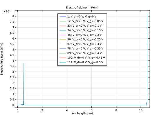
In the Settings window for Line Graph, click Replace Expression in the upper-right corner of the y-Axis Data section. From the menu, choose Component 1 (comp1) > Electrostatics > Electric > es.normE - Electric field norm - V/m.
3
Click to expand the Legends section. Select the Show legends checkbox.
4
In the E-y toolbar, click  Plot.
h-y
1
In the Model Builder window, right-click E-y and choose Duplicate.
2
In the Settings window for 1D Plot Group, type h-y in the Label text field.
Line Graph 1
1
In the Model Builder window, expand the h-y node, then click Line Graph 1.
2
In the Settings window for Line Graph, locate the y-Axis Data section.
3
In the Expression text field, type h.
4
In the h-y toolbar, click  Plot.
5
Click the  y-Axis Log Scale button in the Graphics toolbar.
p-y
1
In the Model Builder window, right-click h-y and choose Duplicate.
2
In the Settings window for 1D Plot Group, type p-y in the Label text field.
Line Graph 1
1
In the Model Builder window, expand the p-y node, then click Line Graph 1.
2
In the Settings window for Line Graph, locate the y-Axis Data section.
3
In the Expression text field, type p.
4
In the p-y toolbar, click  Plot.
n-y
1
In the Model Builder window, right-click p-y and choose Duplicate.
2
In the Settings window for 1D Plot Group, type n-y in the Label text field.
Line Graph 1
1
In the Model Builder window, expand the n-y node, then click Line Graph 1.
2
In the Settings window for Line Graph, locate the y-Axis Data section.
3
In the Expression text field, type n.
4
In the n-y toolbar, click  Plot.
I_dr-V_dr
1
In the Results toolbar, click  1D Plot Group.
2
In the Settings window for 1D Plot Group, type I_dr-V_dr in the Label text field.
3
Locate the Data section. From the Parameter selection (V_g) list, choose Manual.
4
Click  Range.
5
In the Integer Range dialog, type 2 in the Step text field.
6
In the Stop text field, type 11.
7
Click Replace.
Global 1
1
Right-click I_dr-V_dr and choose Global.
2
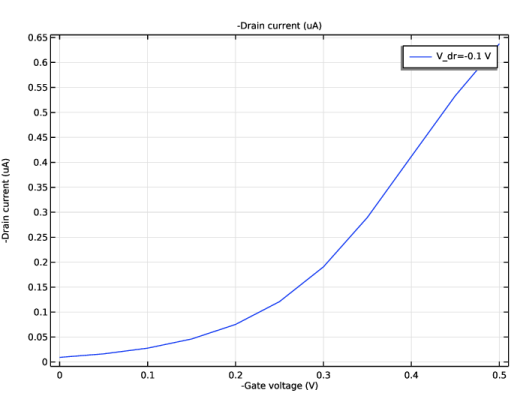
In the Settings window for Global, click Replace Expression in the upper-right corner of the y-Axis Data section. From the menu, choose Component 1 (comp1) > Transport of Holes > Electric > tcc.I0_0 - Conduction current - A.
3
Locate the y-Axis Data section. In the table, enter the following settings:
4
Locate the x-Axis Data section. From the Parameter list, choose Expression.
5
In the Expression text field, type -V_dr.
6
Select the Description checkbox. In the associated text field, type -Drain voltage.
7
Click to expand the Legends section. Find the Include subsection. Clear the Description checkbox.
8
In the I_dr-V_dr toolbar, click  Plot.
I_dr-V_g
1
In the Model Builder window, right-click I_dr-V_dr and choose Duplicate.
2
In the Settings window for 1D Plot Group, type I_dr-V_g in the Label text field.
3
Locate the Data section. From the Parameter selection (V_g) list, choose All.
4
From the Parameter selection (V_dr) list, choose From list.
5
In the Parameter values (V_dr (V)) list box, select -0.1.
Global 1
1
In the Model Builder window, expand the I_dr-V_g node, then click Global 1.
2
In the Settings window for Global, locate the x-Axis Data section.
3
From the Axis source data list, choose V_g.
4
In the Expression text field, type -V_g.
5
In the Description text field, type -Gate voltage.
6
In the I_dr-V_g toolbar, click  Plot.