PDF

Topology Optimization of a Step Thrust Bearing
Introduction
This model is inspired by the Step Thrust Bearing model. In this example, topology optimization will be applied to identify the optimal number grooves and pads as well as their optimal shape.
Model Definition
The geometry and mesh is fixed as is the norm for topology optimization. The out-of-plane geometry is defined in terms of a spatially varying bearing clearance. Topology optimization is performed by letting the variables from the Density Model feature control this clearance. The load capacity of the bearing is a built-in variable, and this is used as objective function. The model is unconstrained and there is no need for projection or special material interpolation, because the problem is self-penalizing for the chosen objective. Regularization is not needed either, but a Helmholtz filter does give smoother results in postprocessing, so this is enabled. See Topology Optimization of an MBB Beam in the Optimization Module Application Library for more details.
Results and Discussion
The topology optimized design is shown in Figure 1 below.
Figure 1: The topology optimized step thrust bearing with grooves (blue) and pads (red).
The optimization finds a design with four grooves when it is initialized with a uniform design. To investigate whether this is indeed the global optimum, the optimization is started with different nonuniform designs to provoke local optima corresponding to three and five grooves. Comparing the performance shows that the design with four grooves has the highest objective function, see Figure 2.
Figure 2: The optimized bearing capacity is plotted versus the number of grooves.
Note that the optimization results in a design specific to the chosen rotation direction. Some practical applications will require that both directions are taken into account, so that symmetry with respect to the rotation can be achieved.
Notes About the COMSOL Implementation
The model demonstrates verification on a body fitted mesh in a new component, as this is good practice for topology optimization. The performance is slightly better with the body fitted mesh.
The model indicates that four grooves is the optimal topology, but running the optimization with a finer mesh and a higher projection slope can give different topologies with significantly better performance (N=1, beta=8, meshsz=1[mm] is one example). This design is qualitatively identical to the design with four grooves, but the ratio between the length and width of the grooves is significantly higher than what is seen in common bearing designs.
Application Library path: Rotordynamics_Module/Optimization/step_thrust_bearing_topology_optimization
Modeling Instructions
From the File menu, choose New.
New
In the New window, click  Model Wizard.
Model Wizard
1
In the Model Wizard window, click  3D.
2
In the Select Physics tree, select Structural Mechanics > Rotordynamics > Hydrodynamic Bearing (hdb).
3
Click Add.
4
Click  Study.
5
In the Select Study tree, select General Studies > Stationary.
6
Geometry 1
Start by importing the parameters for the thrust bearing.
Global Definitions
Parameters 1
1
In the Model Builder window, under Global Definitions click Parameters 1.
2
In the Settings window for Parameters, locate the Parameters section.
3
Click  Load from File.
4
Browse to the model’s Application Libraries folder and double-click the file step_thrust_bearing_topology_optimization_parameters.txt.
Next, create the geometry for the bearing. While doing so, define selections for later use.
Geometry 1
Work Plane 1 (wp1)
In the Geometry toolbar, click  Work Plane.
Work Plane 1 (wp1) > Plane Geometry
In the Model Builder window, click Plane Geometry.
Work Plane 1 (wp1) > Circle 1 (c1)
1
In the Work Plane toolbar, click  Circle.
2
In the Settings window for Circle, locate the Size and Shape section.
3
In the Radius text field, type Ro.
4
Click  Build Selected.
Work Plane 1 (wp1) > Circle 2 (c2)
1
Right-click Component 1 (comp1) > Geometry 1 > Work Plane 1 (wp1) > Plane Geometry > Circle 1 (c1) and choose Duplicate.
2
In the Settings window for Circle, locate the Size and Shape section.
3
In the Radius text field, type Ri.
Work Plane 1 (wp1) > Difference 1 (dif1)
1
In the Work Plane toolbar, click  Booleans and Partitions and choose Difference.
2
3
In the Settings window for Difference, locate the Difference section.
4
Click to select the  Activate Selection toggle button for Objects to subtract.
5
6
Click  Build Selected.
Work Plane 1 (wp1) > Line Segment 1 (ls1)
1
In the Work Plane toolbar, click  More Primitives and choose Line Segment.
2
On the object dif1, select Point 1 only.
3
In the Settings window for Line Segment, locate the Endpoint section.
4
Click to select the  Activate Selection toggle button for End vertex.
5
On the object dif1, select Point 8 only.
6
Click  Build Selected.
Work Plane 1 (wp1) > Partition Objects 1 (par1)
1
In the Work Plane toolbar, click  Booleans and Partitions and choose Partition Objects.
2
3
In the Settings window for Partition Objects, locate the Partition Objects section.
4
Click to select the  Activate Selection toggle button for Tool objects.
5
6
Click  Build Selected.
Work Plane 1 (wp1)
1
In the Model Builder window, under Component 1 (comp1) > Geometry 1 click Work Plane 1 (wp1).
2
In the Settings window for Work Plane, locate the Selections of Resulting Entities section.
3
Select the Resulting objects selection checkbox.
Interior Edges
1
In the Geometry toolbar, click  Selections and choose Adjacent Selection.
2
In the Settings window for Adjacent Selection, locate the Input Entities section.
3
From the Geometric entity level list, choose Boundary.
4
5
In the Add dialog, select Work Plane 1 in the Input selections list.
6
7
In the Settings window for Adjacent Selection, locate the Output Entities section.
8
From the Geometric entity level list, choose Adjacent edges.
9
From the Exterior edges list, choose None.
10
Select the Interior edges checkbox.
11
In the Label text field, type Interior Edges.
Circumferential Edges
1
In the Geometry toolbar, click  Selections and choose Complement Selection.
2
In the Settings window for Complement Selection, type Circumferential Edges in the Label text field.
3
Locate the Geometric Entity Level section. From the Level list, choose Edge.
4
Locate the Input Entities section. Click  Add.
5
In the Add dialog, select Interior Edges in the Selections to invert list.
6
Materials
Material 1 (mat1)
In the Model Builder window, under Component 1 (comp1) right-click Materials and choose Blank Material.
Hydrodynamic Bearing (hdb)
1
Click the  Show More Options button in the Model Builder toolbar.
2
In the Show More Options dialog, in the tree, select the checkbox for the node Physics > Advanced Physics Options.
3
4
In the Settings window for Hydrodynamic Bearing, locate the Physical Model section.
5
From the Fluid type list, choose Liquid with cavitation.
Materials
1
In the Model Builder window, under Component 1 (comp1) > Materials click Material 1 (mat1).
2
In the Settings window for Material, locate the Material Contents section.
3
Add a Topology Optimization node to optimize the shape of the pads.
Component 1 (comp1)
Density Model 1 (dtopo1)
1
In the Physics toolbar, click  Optimization and choose Topology Optimization.
2
In the Settings window for Density Model, locate the Geometric Entity Selection section.
3
From the Geometric entity level list, choose Boundary.
4
From the Selection list, choose All boundaries.
5
Locate the Projection section. From the Projection type list, choose Hyperbolic tangent projection.
6
In the β text field, type beta.
7
Locate the Interpolation section. From the Interpolation type list, choose Linear.
8
Locate the Control Variable Discretization section. From the Element order list, choose Constant.
Define a nonuniform initial value, so that the optimization can be started close to different local optima.
9
Locate the Control Variable Initial Value section. In the θ0 text field, type if(initUniform,volfrac,0.5+0.5*sin(N*atan2(Yg,Xg))).
Hydrodynamic Bearing (hdb)
Hydrodynamic Thrust Bearing 1
1
In the Physics toolbar, click  Boundaries and choose Hydrodynamic Thrust Bearing.
2
In the Settings window for Hydrodynamic Thrust Bearing, locate the Boundary Selection section.
3
From the Selection list, choose All boundaries.
4
Locate the Reference Surface Properties section. From the Reference normal orientation list, choose Opposite direction to geometry normal.
5
Locate the Bearing Properties section. From the Bearing type list, choose User defined.
6
In the hb1 text field, type hg+hf*dtopo1.theta_p.
7
From the Xc list, choose From geometry.
8
Locate the Collar Properties section. In the Ω text field, type speed.
9
Locate the Fluid Properties section. In the ρc text field, type rho_c.
Bearing Orientation 1
1
In the Model Builder window, click Bearing Orientation 1.
2
In the Settings window for Bearing Orientation, locate the Bearing Orientation section.
3
From the Axis list, choose z-axis.
4
Specify the V vector as
Mesh 1
Mapped 1
1
In the Mesh toolbar, click  More Generators and choose Mapped.
2
In the Settings window for Mapped, locate the Boundary Selection section.
3
From the Selection list, choose All boundaries.
Size
1
In the Model Builder window, click Size.
2
In the Settings window for Size, locate the Element Size section.
3
From the Predefined list, choose Extremely fine.
4
Click  Build All.
5
Click the Custom button.
6
Locate the Element Size Parameters section. In the Maximum element size text field, type meshsz.
7
In the Minimum element size text field, type meshsz/2.
8
Click  Build All.
Study 1
Topology Optimization
1
In the Study toolbar, click  Optimization and choose Topology Optimization.
2
In the Model Builder window, click Study 1.
3
In the Settings window for Study, type Study: Sweep Initial Condition in the Label text field.
Add a Parametric Sweep for the number of pads, initial density distribution of the pad profile, mesh size, and projection slope.
Parametric Sweep
1
In the Study toolbar, click  Parametric Sweep.
2
In the Settings window for Parametric Sweep, locate the Study Settings section.
3
Click  Add twice.
4
Topology Optimization
1
In the Model Builder window, click Topology Optimization.
2
In the Settings window for Topology Optimization, click Replace Expression in the upper-right corner of the Objective Function section. From the menu, choose Component 1 (comp1) > Hydrodynamic Bearing > Fluid loads > Fluid load on collar - N > comp1.hdb.htb1.Fcz - Fluid load on collar, z-component.
Scale the objective for better behavior of the optimization solver.
3
Locate the Objective Function section. Find the Objective settings subsection. From the Objective scaling list, choose Initial solution based.
4
From the Type list, choose Maximization.
Initialize the study to generate plots to show while solving.
5
In the Study toolbar, click  Get Initial Value.
Results
Output material volume factor
1
In the Model Builder window, expand the Topology Optimization node, then click Output material volume factor.
2
In the Settings window for 3D Plot Group, locate the Data section.
3
From the Dataset list, choose Study: Sweep Initial Condition/Solution 1 (sol1).
4
Click the  Go to XY View button in the Graphics toolbar, so that the plot updates while optimizing.
Study: Sweep Initial Condition
Topology Optimization
1
In the Model Builder window, under Study: Sweep Initial Condition click Topology Optimization.
2
In the Settings window for Topology Optimization, click to expand the Output section.
3
Select the Plot checkbox.
4
5
In the Study toolbar, click  Compute.
The default plots show the pressure in the bearing, volume fraction, and optimization threshold.
Results
Fluid Pressure (hdb)
1
Click the  Go to XY View button in the Graphics toolbar.
2
In the Settings window for 3D Plot Group, locate the Data section.
3
From the Parameter value (N,initUniform) list, choose 1: N=3, initUniform=1.
4
In the Fluid Pressure (hdb) toolbar, click  Plot.
1D Plot Group 4
1
In the Model Builder window, expand the Results > Topology Optimization node.
2
Right-click Results and choose 1D Plot Group.
Surface 1
1
In the Model Builder window, expand the Output material volume factor node, then click Surface 1.
2
In the Settings window for Surface, locate the Coloring and Style section.
3
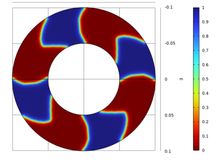
From the Color table transformation list, choose Reverse, so that the thicker oil layer becomes blue.
Output material volume factor
1
In the Model Builder window, click Output material volume factor.
2
In the Settings window for 3D Plot Group, locate the Data section.
3
From the Dataset list, choose Study: Sweep Initial Condition/Parametric Solutions 1 (sol2).
4
From the Parameter value (N,initUniform) list, choose 3: N=4, initUniform=0 to show the best design.
5
In the Output material volume factor toolbar, click  Plot.
6
From the Dataset list, choose Study: Sweep Initial Condition/Solution 1 (sol1), so that the plot still updates while optimizing.
Threshold
You can plot the bearing load capacity versus number of pads for the optimized shape of the bearings. Use the instructions below to generate this plot.
Bearing Capacity vs. Number of Pads
1
In the Model Builder window, under Results click 1D Plot Group 4.
2
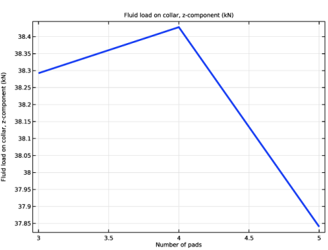
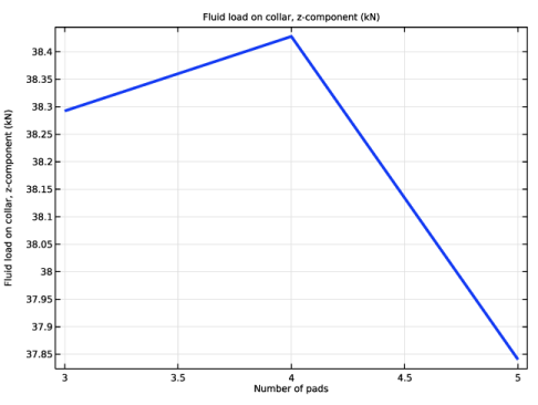
In the Settings window for 1D Plot Group, type Bearing Capacity vs. Number of Pads in the Label text field.
3
Locate the Data section. From the Dataset list, choose Study: Sweep Initial Condition/Parametric Solutions 1 (sol2).
4
From the Parameter selection (N, initUniform) list, choose From list.
5
In the Parameter values (N,initUniform) list, choose 2: N=3, initUniform=0, 3: N=4, initUniform=0, and 4: N=5, initUniform=0.
Global 1
1
Right-click Bearing Capacity vs. Number of Pads and choose Global.
2
In the Settings window for Global, click Replace Expression in the upper-right corner of the y-Axis Data section. From the menu, choose Component 1 (comp1) > Hydrodynamic Bearing > Fluid loads > Fluid load on collar - N > hdb.htb1.Fcz - Fluid load on collar, z-component.
3
Locate the y-Axis Data section. In the table, enter the following settings:
4
Locate the x-Axis Data section. From the Parameter list, choose Expression.
5
In the Expression text field, type N.
6
Click to expand the Coloring and Style section. From the Width list, choose 3.
Bearing Capacity vs. Number of Pads
1
In the Model Builder window, click Bearing Capacity vs. Number of Pads.
2
In the Settings window for 1D Plot Group, locate the Legend section.
3
Clear the Show legends checkbox.
The performance seems to peak for four grooves. You can see that this a numerical effect by running the optimization with meshsz= 1[mm], beta=8, N=16. This gives a better objective, but the design is very different from conventional bearings. In the following we perform a verification in a new component, as this good practice in the context of topology optimization.
Mesh Import Parameters 1
1
In the Model Builder window, expand the Results > Datasets node.
2
Right-click Filter and choose Mesh Import Parameters.
3
In the Settings window for Mesh Import Parameters, locate the Data section.
4
From the Parameter value (N,initUniform) list, choose 3: N=4, initUniform=0.
Filter
Right-click Filter and choose Create Mesh Part.
Mesh Part 1
Import 1
1
In the Settings window for Import, locate the Import section.
2
From the Boundary partitioning list, choose Minimal.
3
Click Import.
Add Component
In the Model Builder window, right-click the root node and choose Add Component > 3D.
Component 1: Optimization
In the Settings window for Component, type Component 1: Optimization in the Label text field.
Component 2: Verification
1
In the Model Builder window, click Component 2 (comp2).
2
In the Settings window for Component, type Component 2: Verification in the Label text field.
Geometry 2
Import 1 (imp1)
1
In the Geometry toolbar, click  Import.
2
In the Settings window for Import, locate the Source section.
3
From the Source list, choose Geometry sequence.
4
From the Geometry list, choose Geometry 1.
Grooves
1
Right-click Import 1 (imp1) and choose Duplicate.
2
In the Settings window for Import, type Grooves in the Label text field.
3
Locate the Source section. From the Source list, choose Mesh or 3D printing file (STL, 3MF, PLY).
4
From the Mesh list, choose Mesh Part 1.
5
Locate the Simplify and Repair section. Clear the Simplify mesh checkbox.
6
Clear the Form solids from surface objects checkbox.
7
Click to expand the Selections of Resulting Entities section. Select the Resulting objects selection checkbox.
8
From the Show in physics list, choose Boundary selection.
Form Union (fin)
1
In the Model Builder window, click Form Union (fin).
2
In the Settings window for Form Union/Assembly, locate the Form Union/Assembly section.
3
From the Repair tolerance list, choose Relative.
4
In the Relative repair tolerance text field, type 1.0E-4.
5
Click  Build Selected.
Pads
1
In the Geometry toolbar, click  Selections and choose Complement Selection.
2
In the Settings window for Complement Selection, type Pads in the Label text field.
3
Locate the Geometric Entity Level section. From the Level list, choose Boundary.
4
Locate the Input Entities section. Click  Add.
5
In the Add dialog, select Grooves in the Selections to invert list.
6
Definitions (comp2)
Groove Variables
1
In the Model Builder window, under Component 2: Verification (comp2) right-click Definitions and choose Variables.
2
In the Settings window for Variables, type Groove Variables in the Label text field.
3
Locate the Geometric Entity Selection section. From the Geometric entity level list, choose Boundary.
4
From the Selection list, choose Grooves.
5
Locate the Variables section. In the table, enter the following settings:
Pad Variables
1
Right-click Groove Variables and choose Duplicate.
2
In the Settings window for Variables, type Pad Variables in the Label text field.
3
Locate the Geometric Entity Selection section. From the Selection list, choose Pads.
4
Locate the Variables section. In the table, enter the following settings:
Materials
Material 1 (mat1)
In the Model Builder window, under Component 1: Optimization (comp1) > Materials right-click Material 1 (mat1) and choose Copy.
Material 1 (mat2)
In the Model Builder window, under Component 2: Verification (comp2) right-click Materials and choose Paste Material.
Hydrodynamic Bearing (hdb)
In the Model Builder window, under Component 1: Optimization (comp1) right-click Hydrodynamic Bearing (hdb) and choose Copy.
Hydrodynamic Bearing (hdb2)
1
In the Model Builder window, right-click Component 2: Verification (comp2) and choose Paste Hydrodynamic Bearing.
2
In the Messages from Paste dialog, click OK.
Hydrodynamic Thrust Bearing 1
1
In the Model Builder window, expand the Hydrodynamic Bearing (hdb2) node, then click Hydrodynamic Thrust Bearing 1.
2
In the Settings window for Hydrodynamic Thrust Bearing, locate the Bearing Properties section.
3
In the hb1 text field, type hfilm.
Initial Values 1
1
In the Model Builder window, click Initial Values 1.
2
In the Settings window for Initial Values, locate the Initial Values section.
3
In the pfilm text field, type 100000[Pa]*hdb2.max(hdb2.hB1)/(0.1*hdb2.max(hdb2.hB1)+hdb2.hB1).
Mesh 2
Free Triangular 1
1
In the Mesh toolbar, click  More Generators and choose Free Triangular.
2
In the Settings window for Free Triangular, locate the Boundary Selection section.
3
From the Geometric entity level list, choose Remaining.
Size
1
In the Model Builder window, click Size.
2
In the Settings window for Size, click to expand the Element Size Parameters section.
3
In the Maximum element size text field, type meshsz.
4
In the Minimum element size text field, type meshsz/2.
5
In the Curvature factor text field, type 10.
6
Click  Build All.
Add Study
1
In the Home toolbar, click  Add Study to open the Add Study window.
2
Go to the Add Study window.
3
Find the Studies subsection. In the Select Study tree, select General Studies > Stationary.
4
Click the Add Study button in the window toolbar.
5
In the Home toolbar, click  Add Study to close the Add Study window.
Study 2
Step 1: Stationary
1
In the Settings window for Stationary, locate the Physics and Variables Selection section.
2
In the Solve for column of the table, under Component 1: Optimization (comp1), clear the checkboxes for Hydrodynamic Bearing (hdb) and Topology Optimization.
Study: Sweep Initial Condition
1
In the Model Builder window, expand the Study: Sweep Initial Condition node, then click Step 1: Stationary.
2
In the Settings window for Stationary, locate the Physics and Variables Selection section.
3
In the Solve for column of the table, under Component 2: Verification (comp2), clear the checkbox for Hydrodynamic Bearing (hdb2).
Verification
1
In the Model Builder window, click Study 2.
2
In the Settings window for Study, type Verification in the Label text field.
3
In the Study toolbar, click  Compute.
Results
Topology Optimization 1
In the Model Builder window, under Results right-click Topology Optimization 1 and choose Delete.
Objective Comparison
1
In the Results toolbar, click  Evaluation Group.
2
In the Settings window for Evaluation Group, type Objective Comparison in the Label text field.
Global Evaluation 1
1
Right-click Objective Comparison and choose Global Evaluation.
2
In the Settings window for Global Evaluation, click Add Expression in the upper-right corner of the Expressions section. From the menu, choose Component 1 (comp1) > Hydrodynamic Bearing > Fluid loads > Fluid load on collar - N > hdb.htb1.Fcz - Fluid load on collar, z-component.
Global Evaluation 2
1
Right-click Global Evaluation 1 and choose Duplicate.
2
In the Settings window for Global Evaluation, locate the Data section.
3
From the Dataset list, choose Verification/Solution 7 (4) (sol7).
4
Click Replace Expression in the upper-right corner of the Expressions section. From the menu, choose Component 2: Verification (comp2) > Hydrodynamic Bearing > Fluid loads > Fluid load on collar - N > hdb2.htb1.Fcz - Fluid load on collar, z-component.
5
In the Objective Comparison toolbar, click  Evaluate.
The performance is slightly higher for the verification in the new component.