PDF

Step Thrust Bearing
Introduction
In this example the pressure distribution in a step thrust bearing is analyzed. A step thrust bearing consists of a stepped bearing surface on which the end of the shaft rotates. The entire assembly is submerged in a lubricant. A six step thrust bearing is considered in this example. The shaft collar is assumed to be spinning without any axial motion in the bearing. The simulation is performed using the Rotordynamics Module’s Hydrodynamic Bearing interface. This interface solves the Reynolds equation to compute the pressure developed in a thin fluid film.
Model Definition
A six-pad step thrust bearing is considered. The inner and outer pad diameters are 0.1 m and 0.2 m, respectively. The grooves span 15° and have a depth of 200 μm.
The bearing is analyzed under various conditions. This includes a parametric study of the angular speed and the film thickness. Here the angular speed and film thickness are varied in the intervals Ω ∈ [500,1000] rad/s and hfilm ∈ [60,160] μm, respectively.
The bearing geometry is shown in Figure 1 below.
Figure 1: Step thrust bearing geometry.
The effect of cavitation is also included in the computation of the fluid-film pressure distribution. The following fluid properties are needed — the dynamic viscosity, the density at cavitation pressure, and the compressibility. The utilized fluid parameters are summarized in Table 1. The selected values are close to those of lubricating oils used in real bearings.
10-7 Pa-1
Results and Discussion
Figure 2 shows the fluid pressure profile in the bearing for the highest values of angular speed and film thickness.
Figure 2: Fluid-film pressure profile at Ω = 1000 rad/s with a film thickness of 160 μm.
The resulting vertical force on the collar associated with the pressure distribution shown above is 7500 N. This is the load carrying capacity of the bearing at the specified speed.
The mass fraction of the lubricant, which is a measure of the cavitation, is shown in Figure 3. It is clear that amount of cavitation is very small and is localized near the trailing edge of the pads.
Figure 3: Mass fraction at Ω = 1000 rad/s with a film thickness of 160 μm.
The pressure distribution in radial and circumferential directions on a single pad are shown in Figure 4 and Figure 5, respectively. The pressure at the inner and outer radius locations are zero with the distribution marginally biased toward the outer edge. The velocity of the collar varies linearly from the inner to the outer radius. Since the pressure is proportional to the shear velocity in the film, it is expected to increase linearly from the inner point to the outer point. However, along the inner and outer edge the film pressure is set to zero. Therefore, the maximum pressure occurs toward the outer side relative to the mid position. In the circumferential direction, the pressure suddenly rises at the step location, that is, the leading edge of the pad, and reduces slowly toward the trailing edge.
Figure 4: Pressure profiles in radial direction at Ω = 1000 rad/s.
Figure 5: Pressure profiles in circumferential direction at Ω = 1000 rad/s.
Figure 6 shows bearing profile computed using the film thickness.
Figure 6: Bearing profile.
Application Library path: Rotordynamics_Module/Tutorials/step_thrust_bearing
Modeling Instructions
From the File menu, choose New.
New
In the New window, click  Model Wizard.
Model Wizard
1
In the Model Wizard window, click  3D.
2
In the Select Physics tree, select Structural Mechanics > Rotordynamics > Hydrodynamic Bearing (hdb).
3
Click Add.
4
Click  Study.
5
In the Select Study tree, select General Studies > Stationary.
6
Global Definitions
Parameters 1
1
In the Model Builder window, under Global Definitions click Parameters 1.
2
In the Settings window for Parameters, locate the Parameters section.
3
Click  Load from File.
4
Geometry 1
Work Plane 1 (wp1)
In the Geometry toolbar, click  Work Plane.
Work Plane 1 (wp1) > Plane Geometry
In the Model Builder window, click Plane Geometry.
Work Plane 1 (wp1) > Circle 1 (c1)
1
In the Work Plane toolbar, click  Circle.
2
In the Settings window for Circle, locate the Size and Shape section.
3
In the Radius text field, type Ro.
4
Click to expand the Layers section. In the table, enter the following settings:
5
Click  Build Selected.
Work Plane 1 (wp1) > Delete Entities 1 (del1)
1
Right-click Plane Geometry and choose Delete Entities.
2
In the Settings window for Delete Entities, locate the Entities or Objects to Delete section.
3
From the Geometric entity level list, choose Domain.
4
On the object c1, select Domain 5 only.
5
Click  Build Selected.
Hydrodynamic Bearing (hdb)
1
Click the  Show More Options button in the Model Builder toolbar.
2
In the Show More Options dialog, in the tree, select the checkbox for the node Physics > Advanced Physics Options.
3
Enable the Cavitation formulation in the bearing.
4
In the Model Builder window, under Component 1 (comp1) click Hydrodynamic Bearing (hdb).
5
In the Settings window for Hydrodynamic Bearing, locate the Physical Model section.
6
From the Fluid type list, choose Liquid with cavitation.
Reduce the Cavitation transition width for the sharper transition between the cavitated and noncavitated regions.
7
In the Δpsw text field, type 0.5[MPa].
Materials
Material 1 (mat1)
1
In the Model Builder window, under Component 1 (comp1) right-click Materials and choose Blank Material.
2
In the Settings window for Material, locate the Material Contents section.
3
Hydrodynamic Bearing (hdb)
Hydrodynamic Thrust Bearing 1
1
In the Physics toolbar, click  Boundaries and choose Hydrodynamic Thrust Bearing.
2
In the Settings window for Hydrodynamic Thrust Bearing, locate the Boundary Selection section.
3
From the Selection list, choose All boundaries.
Because the reference surface is assumed to be located on the collar, change the Reference normal orientation to align it with the collar normal.
4
Locate the Reference Surface Properties section. From the Reference normal orientation list, choose Opposite direction to geometry normal.
5
Locate the Bearing Properties section. From the Bearing type list, choose Step.
6
In the γp text field, type padAng.
7
In the di text field, type 2*Ri.
8
In the do text field, type 2*Ro.
9
In the hs text field, type hg.
10
In the hfilm text field, type h_film.
11
From the Groove type list, choose Constant arc.
12
Locate the Collar Properties section. In the Ω text field, type angSpeed.
13
Locate the Fluid Properties section. In the ρc text field, type rho_c.
Bearing Orientation 1
1
In the Model Builder window, click Bearing Orientation 1.
2
In the Settings window for Bearing Orientation, locate the Bearing Orientation section.
3
From the Axis list, choose z-axis.
4
Specify the V vector as
5
In the ϕ text field, type gAng.
Initial Values 1
An auxiliary sweep will be used in the stationary study, which does not support parameter dependencies in initial expressions. Therefore, apply a constant initial value for the pressure.
1
In the Model Builder window, click Initial Values 1.
2
In the Settings window for Initial Values, locate the Initial Values section.
3
In the pfilm text field, type 100000[Pa].
Mesh 1
Mapped 1
1
In the Mesh toolbar, click  More Generators and choose Mapped.
2
In the Settings window for Mapped, locate the Boundary Selection section.
3
From the Selection list, choose All boundaries.
Create one element per degree in the azimuthal direction to capture the pressure accurately.
Distribution 1
1
Right-click Mapped 1 and choose Distribution.
2
3
In the Settings window for Distribution, locate the Distribution section.
4
In the Number of elements text field, type 90.
Distribution 2
1
In the Model Builder window, right-click Mapped 1 and choose Distribution.
2
3
In the Settings window for Distribution, locate the Distribution section.
4
In the Number of elements text field, type 20.
5
In the Model Builder window, right-click Mesh 1 and choose Build All.
Study 1
Step 1: Stationary
1
In the Model Builder window, under Study 1 click Step 1: Stationary.
2
In the Settings window for Stationary, click to expand the Study Extensions section.
3
Select the Auxiliary sweep checkbox.
4
5
6
7
8
From the Sweep type list, choose All combinations.
9
In the Study toolbar, click  Compute.
Set preferred units for the pressure by following the instructions below.
Results
Preferred Units 1
1
In the Results toolbar, click  Configurations and choose Preferred Units.
2
In the Settings window for Preferred Units, locate the Units section.
3
Click  Add Physical Quantity.
4
In the Physical Quantity dialog, type pres in the text field.
5
In the tree, select General > Pressure (Pa).
6
7
In the Settings window for Preferred Units, locate the Units section.
8
9
Click  Apply.
Default plot shows the pressure distribution in the bearing. To generate the height plot for the pressure distribution shown in Figure 2 start by creating a Surface dataset.
Surface 1
1
In the Results toolbar, click  More Datasets and choose Surface.
2
In the Settings window for Surface, locate the Selection section.
3
From the Selection list, choose All boundaries.
Fluid Pressure (hdb)
1
In the Model Builder window, under Results click Fluid Pressure (hdb).
2
In the Settings window for 3D Plot Group, click to expand the Title section.
3
From the Title type list, choose Label.
4
Locate the Color Legend section. Select the Show units checkbox.
Pressure (Height)
1
In the Results toolbar, click  2D Plot Group.
2
In the Settings window for 2D Plot Group, type Pressure (Height) in the Label text field.
3
Click to expand the Title section. From the Title type list, choose Label.
4
Locate the Color Legend section. Select the Show units checkbox.
Surface 1
1
Right-click Pressure (Height) and choose Surface.
2
In the Settings window for Surface, locate the Expression section.
3
In the Expression text field, type hdb.p.
4
Locate the Coloring and Style section. From the Color table list, choose Traffic.
Height Expression 1
1
Right-click Surface 1 and choose Height Expression.
2
In the Settings window for Height Expression, locate the Axis section.
3
Select the Scale factor checkbox. In the associated text field, type 2e-3.
4
Click the  Go to Default View button in the Graphics toolbar.
5
In the Pressure (Height) toolbar, click  Plot.
The following instructions are to plot the mass fraction of the lubricant shown in Figure 3.
Mass Fraction
1
In the Home toolbar, click  Add Plot Group and choose 3D Plot Group.
2
In the Settings window for 3D Plot Group, type Mass Fraction in the Label text field.
3
Click to expand the Title section. From the Title type list, choose Label.
Contour 1
1
Right-click Mass Fraction and choose Contour.
2
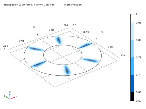
In the Settings window for Contour, click Replace Expression in the upper-right corner of the Expression section. From the menu, choose Component 1 (comp1) > Hydrodynamic Bearing > Cavitation > hdb.theta - Mass fraction - 1.
3
Locate the Coloring and Style section. From the Contour type list, choose Filled.
4
Locate the Levels section. In the Total levels text field, type 5.
5
Locate the Coloring and Style section. From the Color table list, choose JupiterAuroraBorealis.
6
Click the  Go to Default View button in the Graphics toolbar.
7
In the Mass Fraction toolbar, click  Plot.
Figure 6 shows the bearing profile. Follow the instructions below to replicate it.
2D Plot Group 4
In the Results toolbar, click  2D Plot Group.
Surface 1
1
Right-click 2D Plot Group 4 and choose Surface.
2
In the Settings window for Surface, locate the Expression section.
3
In the Expression text field, type hg-hdb.h.
4
Locate the Coloring and Style section. From the Coloring list, choose Uniform.
5
From the Color list, choose Gray.
Height Expression 1
1
Right-click Surface 1 and choose Height Expression.
2
In the Settings window for Height Expression, locate the Axis section.
3
Select the Scale factor checkbox. In the associated text field, type 100.
Pad Profile
1
In the Model Builder window, under Results click 2D Plot Group 4.
2
In the Settings window for 2D Plot Group, type Pad Profile in the Label text field.
3
Click to expand the Title section. From the Title type list, choose Label.
4
Locate the Plot Settings section. Clear the Plot dataset edges checkbox.
5
Click the  Go to Default View button in the Graphics toolbar.
6
In the Pad Profile toolbar, click  Plot.
You can also analyze the pressure distributions along the radial and circumferential directions of the bearing shown in Figure 4 and Figure 5. Start by creating a Cut line along the radial line.
Cut Line 3D: Radial Line
1
In the Results toolbar, click  Cut Line 3D.
2
In the Settings window for Cut Line 3D, locate the Line Data section.
3
In row Point 2, set X to 0.
4
In row Point 2, set Y to Ro.
5
6
In the Label text field, type Cut Line 3D: Radial Line.
Radial Distribution of Pressure (Film Thickness)
1
In the Results toolbar, click  1D Plot Group.
2
In the Settings window for 1D Plot Group, locate the Data section.
3
From the Dataset list, choose Cut Line 3D: Radial Line.
4
From the Parameter selection (angSpeed) list, choose Last.
5
In the Label text field, type Radial Distribution of Pressure (Film Thickness).
6
Click to expand the Title section. From the Title type list, choose Label.
Line Graph 1
1
Right-click Radial Distribution of Pressure (Film Thickness) and choose Line Graph.
2
In the Settings window for Line Graph, locate the y-Axis Data section.
3
In the Expression text field, type hdb.p.
4
Click to expand the Legends section. Select the Show legends checkbox.
5
From the Legends list, choose Evaluated.
6
In the Legend text field, type h = eval(h_film, um) \mu m.
7
In the Radial Distribution of Pressure (Film Thickness) toolbar, click  Plot.
Radial Distribution of Pressure (Film Thickness)
1
In the Model Builder window, click Radial Distribution of Pressure (Film Thickness).
2
In the Settings window for 1D Plot Group, locate the Legend section.
3
From the Position list, choose Upper left.
Radial Distribution of Pressure (Angular Speed)
1
Right-click Radial Distribution of Pressure (Film Thickness) and choose Duplicate.
2
In the Settings window for 1D Plot Group, locate the Data section.
3
From the Parameter selection (h_film) list, choose Last.
4
From the Parameter selection (angSpeed) list, choose All.
5
In the Label text field, type Radial Distribution of Pressure (Angular Speed).
Line Graph 1
1
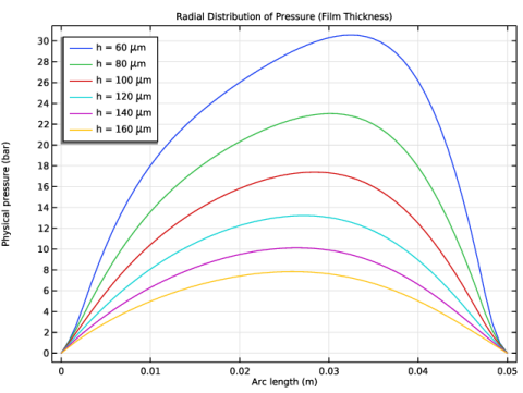
In the Model Builder window, expand the Radial Distribution of Pressure (Angular Speed) node, then click Line Graph 1.
2
In the Settings window for Line Graph, locate the Legends section.
3
In the Legend text field, type \Omega = eval(angSpeed) rad/s.
4
In the Radial Distribution of Pressure (Angular Speed) toolbar, click  Plot.
Radial Distribution of Pressure (Film Thickness)
In the Model Builder window, collapse the Results > Radial Distribution of Pressure (Film Thickness) node.
Use the Parametric Curve to create the circumferential sector line.
Parametric Curve 3D: Circumferential Line
1
In the Results toolbar, click  More Datasets and choose Parametric Curve 3D.
2
In the Settings window for Parametric Curve 3D, locate the Parameter section.
3
In the Maximum text field, type 2*pi/N.
4
Locate the Expressions section. In the x text field, type 0.5*(Ro+Ri)*cos(s).
5
In the y text field, type 0.5*(Ro+Ri)*sin(s).
6
In the Label text field, type Parametric Curve 3D: Circumferential Line.
7
Radial Distribution of Pressure (Angular Speed), Radial Distribution of Pressure (Film Thickness)
1
In the Model Builder window, under Results, Ctrl-click to select Radial Distribution of Pressure (Film Thickness) and Radial Distribution of Pressure (Angular Speed).
2
Circumferential Distribution of Pressure (Film Thickness)
1
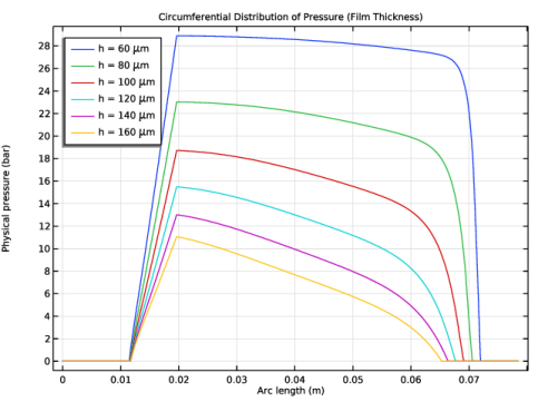
In the Settings window for 1D Plot Group, type Circumferential Distribution of Pressure (Film Thickness) in the Label text field.
2
Locate the Data section. From the Dataset list, choose Parametric Curve 3D: Circumferential Line.
3
In the Circumferential Distribution of Pressure (Film Thickness) toolbar, click  Plot.
Circumferential Distribution of Pressure (Angular Speed)
1
In the Model Builder window, under Results click Radial Distribution of Pressure (Angular Speed) 1.
2
In the Settings window for 1D Plot Group, type Circumferential Distribution of Pressure (Angular Speed) in the Label text field.
3
Locate the Data section. From the Dataset list, choose Parametric Curve 3D: Circumferential Line.
4
Locate the Legend section. From the Position list, choose Upper right.
5
In the Circumferential Distribution of Pressure (Angular Speed) toolbar, click  Plot.
Lift Force
1
In the Results toolbar, click  1D Plot Group.
2
In the Settings window for 1D Plot Group, type Lift Force in the Label text field.
3
Locate the Title section. From the Title type list, choose Label.
Global 1
1
Right-click Lift Force and choose Global.
2
In the Settings window for Global, click Replace Expression in the upper-right corner of the y-Axis Data section. From the menu, choose Component 1 (comp1) > Hydrodynamic Bearing > Fluid loads > Fluid load on collar - N > hdb.htb1.Fcz - Fluid load on collar, z-component.
3
Click to expand the Legends section. Locate the y-Axis Data section. In the table, enter the following settings:
4
Locate the Legends section. From the Legends list, choose Evaluated.
5
In the Legend text field, type h = eval(h_film, um) \mu m.
6
In the Lift Force toolbar, click  Plot.
Lift Force
1
In the Model Builder window, click Lift Force.
2
In the Settings window for 1D Plot Group, locate the Legend section.
3
From the Position list, choose Upper left.
4
Locate the Plot Settings section.
5
Select the x-axis label checkbox. In the associated text field, type Angular speed of the shaft (rad/s).
6
In the Lift Force toolbar, click  Plot.