PDF

Thermal Stress in a Rotor due to Bearing Heat Loss
Introduction
The lubricant in hydrodynamic bearings gets sheared due to the relative velocity between the surfaces of the journal and the bushing, which causes viscous heat dissipation. This heat is conducted to the neighboring journal and bearing housing. Surfaces of the rotor and the housing finally convects this heat to the atmosphere. In a steady state situations, the temperature profile in the system is such that the heat generated in the bearings is equal to the heat convected to the atmosphere. A varying temperature profile in the system causes a thermal deformation as well as thermal stresses.
In this model, a rotor-bearing system is considered to study the thermal equilibrium due to heat dissipation in bearings by performing a stationary analysis. The resulting stresses and deformations are also studied.
Model Definition
The model consists of a rotor supported by two hydrodynamic bearings. The housing of each bearing is also modeled. The rotor is supported by thrust bearings at its ends, and another thrust bearing at the collar on the rotor between both the two journal bearings. The geometry of the system is shown in Figure 1.
Figure 1: Rotor geometry.
Modeling of the problem requires coupling between the different physical phenomena and physics interfaces; these are listed in the following:
Note that the multiphysics interface Thermal Stress, Solid automatically adds the Heat Transfer in Solids and Solid Mechanics interfaces together with the Thermal Expansion multiphysics coupling. Therefore, the multiphysics interface can be used instead of adding them individually.
Heat Convection
The rotor and bearing housings both convect heat to the atmosphere. The housings are stationary and only natural convection takes place. A nominal value of 5 W/(m2·K) is used as a heat transfer coefficient. Heat convection from the rotor is more complicated due to the rotation of the rotor. The heat transfer coefficient for the external surfaces of the rotor is given by
where kair is the thermal conductivity of the air, R is the radius of the rotor, Re,air is the Reynolds number of the rotor given by
where Ω is the angular speed of the rotor, D is the diameter of the rotor and νair is the kinematic viscosity of the air. The Prandtl number, Pr,air, is given by
The properties of the bearing are given in Table 1, and the properties of air in Table 2.
2000 J/kg.K
Table 2: Air properties.
17·10-6 m2/s
This model only considers a unidirectional coupling in which the viscous heat dissipation changes the temperature of the system, causing thermal deformation and stress. In general, viscous heat dissipation can depend on the temperature through the viscosity and density of the lubricant, and on thermal deformation changing the clearance of the bearing. These effects are ignored in this model. They can, however, easily be included by making the lubricant properties functions of temperature and adjusting the bearing clearance to incorporate the change of the gap due to thermal expansion of the materials.
Results and Discussion
The pressure in the bearings is shown in Figure 2. The maximum pressure is located at the bottom of the bearing to support the static load.
Figure 2: Pressure in the bearings.
The viscous heat dissipation in the bearing is shown in Figure 3. The maximum dissipation occurs where the pressure gradient is the largest.
Figure 3: Viscous heat dissipation in the bearings.
The temperature profile in the bearing is shown in Figure 4. Significant heat dissipation occurs only at the location of the minimum film thickness. The temperature profile in the bearing is uniform due to the heat convection through the flow of the lubricant. Note that the temperature in both bearings is slightly different due to asymmetry in the heat convection from the rotor. The temperature in the rotor and the bearing housings is shown in Figure 5.
Figure 4: Temperature in the film.
.
Figure 5: Temperature in the rotor and the bearing housings.
The stress in the rotor and the housings is shown in Figure 6. In the housings, the maximum stress occurs in the connection holes. As the connection holes are fixed, thermal expansion is resisted at these locations. In the rotor, the largest stresses appear near the thrust bearings. The rotor will expand radially as well as axially due the temperature increase, and the axial expansion is restricted by the thrust bearings giving rise to high stresses in these locations.
Figure 6: Stress in the rotor and the bearing housings.
Application Library path: Rotordynamics_Module/Tutorials/rotor_thermal_stress
Modeling Instructions
From the File menu, choose New.
New
In the New window, click  Model Wizard.
Model Wizard
1
In the Model Wizard window, click  3D.
The problem involves the bearing modeling together with heat transfer in the film and heat transfer in the housing and shaft. Add corresponding interfaces to model all the physical phenomena.
2
In the Select Physics tree, select Heat Transfer > Thin Structures > Heat Transfer in Films (htlsh), Structural Mechanics > Rotordynamics > Hydrodynamic Bearing (hdb), and Structural Mechanics > Thermal–Structure Interaction > Thermal Stress, Solid.
3
Click Add.
4
Click  Study.
5
In the Select Study tree, select General Studies > Stationary.
6
Geometry 1
Import 1 (imp1)
1
In the Geometry toolbar, click  Import.
2
In the Settings window for Import, locate the Source section.
3
Click  Browse.
4
5
Click  Import.
Form Union (fin)
1
In the Model Builder window, under Component 1 (comp1) > Geometry 1 click Form Union (fin).
2
In the Settings window for Form Union/Assembly, locate the Form Union/Assembly section.
3
From the Action list, choose Form an assembly.
Create an imprint on the shaft to use it as journal surface.
4
Select the Create imprints checkbox.
5
In the Geometry toolbar, click  Build All.
Disable the analysis of the geometry as the remaining small geometric details can be kept.
6
In the Model Builder window, click Geometry 1.
7
In the Settings window for Geometry, locate the Cleanup section.
8
Clear the Automatic detection of small details checkbox.
Global Definitions
Parameters 1
1
In the Model Builder window, under Global Definitions click Parameters 1.
2
In the Settings window for Parameters, locate the Parameters section.
3
Click  Load from File.
4
Create some selections for later use.
Definitions
Bearing Housing
1
In the Definitions toolbar, click  Explicit.
2
3
In the Settings window for Explicit, type Bearing Housing in the Label text field.
Rotor
1
In the Definitions toolbar, click  Complement.
2
In the Settings window for Complement, type Rotor in the Label text field.
3
Locate the Input Entities section. Under Selections to invert, click  Add.
4
In the Add dialog, select Bearing Housing in the Selections to invert list.
5
Identity Boundary Pair 1 (ap1)
1
In the Model Builder window, under Component 1 (comp1) > Definitions click Identity Boundary Pair 1 (ap1).
2
In the Settings window for Pair, locate the Source Boundaries section.
3
Click  Create Selection.
4
In the Create Selection dialog, type Journal 1 in the Selection name text field.
5
6
In the Settings window for Pair, locate the Destination Boundaries section.
7
Click  Create Selection.
8
In the Create Selection dialog, type Bearing 1 in the Selection name text field.
9
Identity Boundary Pair 2 (ap2)
1
In the Model Builder window, click Identity Boundary Pair 2 (ap2).
2
In the Settings window for Pair, locate the Source Boundaries section.
3
Click  Create Selection.
4
In the Create Selection dialog, type Journal 2 in the Selection name text field.
5
6
In the Settings window for Pair, locate the Destination Boundaries section.
7
Click  Create Selection.
8
In the Create Selection dialog, type Bearing 2 in the Selection name text field.
9
Housing foundation
1
In the Definitions toolbar, click  Explicit.
2
In the Settings window for Explicit, type Housing foundation in the Label text field.
3
Locate the Input Entities section. From the Geometric entity level list, choose Boundary.
4
5
Select the Group by continuous tangent checkbox.
Journals
1
In the Definitions toolbar, click  Union.
2
In the Settings window for Union, type Journals in the Label text field.
3
Locate the Geometric Entity Level section. From the Level list, choose Boundary.
4
Locate the Input Entities section. Under Selections to add, click  Add.
5
In the Add dialog, in the Selections to add list, choose Journal 1 and Journal 2.
6
Bearings
1
In the Definitions toolbar, click  Union.
2
In the Settings window for Union, type Bearings in the Label text field.
3
Locate the Geometric Entity Level section. From the Level list, choose Boundary.
4
Locate the Input Entities section. Under Selections to add, click  Add.
5
In the Add dialog, in the Selections to add list, choose Bearing 1 and Bearing 2.
6
Shaft Exterior
1
In the Definitions toolbar, click  Adjacent.
2
In the Settings window for Adjacent, locate the Input Entities section.
3
Under Input selections, click  Add.
4
In the Add dialog, select Rotor in the Input selections list.
5
6
In the Settings window for Adjacent, type Shaft Exterior in the Label text field.
Housing Exterior
1
Right-click Shaft Exterior and choose Duplicate.
2
In the Settings window for Adjacent, locate the Input Entities section.
3
In the Input selections list box, select Rotor.
4
Under Input selections, click  Delete.
5
Under Input selections, click  Add.
6
In the Add dialog, select Bearing Housing in the Input selections list.
7
8
In the Settings window for Adjacent, type Housing Exterior in the Label text field.
Convective boundaries (Shaft)
1
In the Definitions toolbar, click  Difference.
2
In the Settings window for Difference, locate the Geometric Entity Level section.
3
From the Level list, choose Boundary.
4
Locate the Input Entities section. Under Selections to add, click  Add.
5
In the Add dialog, select Shaft Exterior in the Selections to add list.
6
7
In the Settings window for Difference, locate the Input Entities section.
8
Under Selections to subtract, click  Add.
9
In the Add dialog, select Journals in the Selections to subtract list.
10
11
In the Settings window for Difference, type Convective boundaries (Shaft) in the Label text field.
Convective boundaries (Housing)
1
Right-click Convective boundaries (Shaft) and choose Duplicate.
2
In the Settings window for Difference, type Convective boundaries (Housing) in the Label text field.
3
Locate the Input Entities section. In the Selections to add list box, select Shaft Exterior.
4
Under Selections to add, click  Delete.
5
Under Selections to add, click  Add.
6
In the Add dialog, select Housing Exterior in the Selections to add list.
7
8
In the Settings window for Difference, locate the Input Entities section.
9
In the Selections to subtract list box, select Journals.
10
Under Selections to subtract, click  Delete.
11
Under Selections to subtract, click  Add.
12
In the Add dialog, select Bearings in the Selections to subtract list.
13
Exterior Edges (Journal)
1
In the Definitions toolbar, click  Adjacent.
2
In the Settings window for Adjacent, locate the Input Entities section.
3
From the Geometric entity level list, choose Boundary.
4
Under Input selections, click  Add.
5
In the Add dialog, select Journals in the Input selections list.
6
7
In the Settings window for Adjacent, locate the Output Entities section.
8
From the Geometric entity level list, choose Adjacent edges.
9
In the Label text field, type Exterior Edges (Journal).
Interior Edges (Journal)
1
Right-click Exterior Edges (Journal) and choose Duplicate.
2
In the Settings window for Adjacent, type Interior Edges (Journal) in the Label text field.
3
Locate the Output Entities section. From the Exterior edges list, choose None.
4
Select the Interior edges checkbox.
Create variable for convection coefficient on the shaft surface.
Variables 1
1
In the Model Builder window, right-click Definitions and choose Variables.
2
In the Settings window for Variables, locate the Geometric Entity Selection section.
3
From the Geometric entity level list, choose Boundary.
4
From the Selection list, choose Convective boundaries (Shaft).
5
Locate the Variables section. In the table, enter the following settings:
Add a General Extrusion operator to pick the temperature of the housing as a boundary temperature in lubricant film.
General Extrusion 1 (genext1)
1
In the Definitions toolbar, click  Nonlocal Couplings and choose General Extrusion.
2
In the Settings window for General Extrusion, locate the Source Selection section.
3
From the Geometric entity level list, choose Boundary.
4
From the Selection list, choose Bearings.
5
Locate the Destination Map section. In the x-expression text field, type X.
6
In the y-expression text field, type Y.
7
In the z-expression text field, type Z.
8
Locate the Source section. From the Source frame list, choose Material  (X, Y, Z).
Add Material
1
In the Materials toolbar, click  Add Material to open the Add Material window.
2
Go to the Add Material window.
3
In the tree, select Built-in > Structural steel.
4
Click the Add to Component button in the window toolbar.
5
In the Materials toolbar, click  Add Material to close the Add Material window.
Materials
Material 2 (mat2)
1
In the Model Builder window, under Component 1 (comp1) right-click Materials and choose Blank Material.
2
In the Settings window for Material, locate the Geometric Entity Selection section.
3
From the Geometric entity level list, choose Boundary.
4
From the Selection list, choose Journals.
Heat Transfer in Films (htlsh)
1
In the Model Builder window, under Component 1 (comp1) click Heat Transfer in Films (htlsh).
2
In the Settings window for Heat Transfer in Films, locate the Boundary Selection section.
3
From the Selection list, choose Journals.
Hydrodynamic Bearing (hdb)
1
In the Model Builder window, under Component 1 (comp1) click Hydrodynamic Bearing (hdb).
2
In the Settings window for Hydrodynamic Bearing, locate the Boundary Selection section.
3
From the Selection list, choose Journals.
Materials
1
In the Model Builder window, under Component 1 (comp1) > Materials click Material 2 (mat2).
2
In the Settings window for Material, locate the Material Contents section.
3
4
In the Label text field, type Material: Oil.
Heat Transfer in Films (htlsh)
Fluid 1
1
In the Model Builder window, under Component 1 (comp1) > Heat Transfer in Films (htlsh) click Fluid 1.
2
In the Settings window for Fluid, locate the Layer Model section.
3
From the Layer type list, choose General.
Use the mean flow velocity of the film as a convective velocity for the heat transfer.
4
Locate the Heat Convection section. From the u list, choose Mean fluid velocity (material frame) (hdb/hjb1).
Heat Source 1
1
In the Physics toolbar, click  Boundaries and choose Heat Source.
2
In the Settings window for Heat Source, locate the Boundary Selection section.
3
From the Selection list, choose Journals.
Use the viscous heat dissipation from bearing as a heat source in the film.
4
Locate the Heat Source section. From the Q0 list, choose Viscous dissipation (hdb/hjb1).
Temperature is continuous between the lubricant film and the surrounding boundaries in contact with the film. Assign the temperature from the shaft as temperature at the top interface of the film. Similarly, assign the temperature of the housing as the temperature at the bottom interface of the film.
Temperature, Interface 1
1
In the Physics toolbar, click  Boundaries and choose Temperature, Interface.
2
In the Settings window for Temperature, Interface, locate the Interface Selection section.
3
From the Apply to list, choose Top interface.
4
Locate the Temperature section. In the T0 text field, type T2.
5
Locate the Boundary Selection section. From the Selection list, choose Journals.
Temperature, Interface 2
1
Right-click Temperature, Interface 1 and choose Duplicate.
2
In the Settings window for Temperature, Interface, locate the Interface Selection section.
3
From the Apply to list, choose Bottom interface.
4
Locate the Temperature section. In the T0 text field, type genext1(T2).
Since, the film is modeled on the journal boundary, a General Extrusion operator is used to pick the temperature from the housing boundary.
Hydrodynamic Bearing (hdb)
1
Click the  Show More Options button in the Model Builder toolbar.
2
In the Show More Options dialog, in the tree, select the checkbox for the node Physics > Advanced Physics Options.
3
4
In the Model Builder window, under Component 1 (comp1) click Hydrodynamic Bearing (hdb).
5
In the Settings window for Hydrodynamic Bearing, locate the Physical Model section.
6
From the Fluid type list, choose Liquid with cavitation.
Hydrodynamic Journal Bearing 1
1
In the Model Builder window, under Component 1 (comp1) > Hydrodynamic Bearing (hdb) click Hydrodynamic Journal Bearing 1.
2
In the Settings window for Hydrodynamic Journal Bearing, locate the Bearing Properties section.
3
In the C text field, type C.
4
From the Xc list, choose From geometry.
Bearing pressure supports the static load on the shaft. Assign half of the static load in each bearing.
5
Locate the Journal Properties section. From the Specify list, choose Load.
6
Specify the Wj vector as
7
In the Ω text field, type 2*pi[rad]*fr.
Duplicate the current feature and change the selection to model the second bearing.
Hydrodynamic Journal Bearing 2
1
Right-click Component 1 (comp1) > Hydrodynamic Bearing (hdb) > Hydrodynamic Journal Bearing 1 and choose Duplicate.
2
In the Settings window for Hydrodynamic Journal Bearing, locate the Boundary Selection section.
3
From the Selection list, choose Journal 2.
Bearing Orientation 1
1
In the Model Builder window, click Bearing Orientation 1.
2
In the Settings window for Bearing Orientation, locate the Bearing Orientation section.
3
From the Axis list, choose y-axis.
4
Specify the V vector as
Solid Mechanics (solid)
In the Model Builder window, under Component 1 (comp1) click Solid Mechanics (solid).
Fixed Constraint 1
1
In the Physics toolbar, click  Boundaries and choose Fixed Constraint.
2
In the Settings window for Fixed Constraint, locate the Boundary Selection section.
3
From the Selection list, choose Housing foundation.
Add a Prescribed Displacement to model the thrust bearings. Two of the thrust bearings are at rotor ends and one is located in between the journal bearings at collars.
Prescribed Displacement 1
1
In the Physics toolbar, click  Boundaries and choose Prescribed Displacement.
2
3
In the Settings window for Prescribed Displacement, locate the Prescribed Displacement section.
4
From the Displacement in y direction list, choose Prescribed.
Add another Prescribed Displacement node at the axial edges of the rotor in the journal bearings. This is to restrict the motion of the rotor in the lateral directions at the bearing locations.
Prescribed Displacement 2
1
In the Physics toolbar, click  Edges and choose Prescribed Displacement.
2
3
In the Settings window for Prescribed Displacement, locate the Prescribed Displacement section.
4
From the Displacement in x direction list, choose Prescribed.
5
From the Displacement in z direction list, choose Prescribed.
Heat Transfer in Solids (ht)
In the Model Builder window, under Component 1 (comp1) click Heat Transfer in Solids (ht).
Heat Flux: Shaft
1
In the Physics toolbar, click  Boundaries and choose Heat Flux.
2
In the Settings window for Heat Flux, type Heat Flux: Shaft in the Label text field.
3
Locate the Boundary Selection section. From the Selection list, choose Convective boundaries (Shaft).
4
Locate the Heat Flux section. From the Flux type list, choose Convective heat flux.
5
In the h text field, type h_shaft.
Heat Flux: Housing
1
Right-click Heat Flux: Shaft and choose Duplicate.
2
In the Settings window for Heat Flux, type Heat Flux: Housing in the Label text field.
3
Locate the Boundary Selection section. From the Selection list, choose Convective boundaries (Housing).
4
Locate the Heat Flux section. In the h text field, type 5.
Mesh 1
Identical Mesh 1
1
In the Mesh toolbar, click  More Attributes and choose Identical Mesh.
2
In the Settings window for Identical Mesh, locate the First Entity Group section.
3
From the Selection list, choose Journals.
4
Locate the Second Entity Group section. From the Selection list, choose Bearings.
Swept 1
1
In the Mesh toolbar, click  Swept.
2
In the Settings window for Swept, locate the Domain Selection section.
3
From the Geometric entity level list, choose Domain.
4
From the Selection list, choose Rotor.
Distribution 1
1
Right-click Swept 1 and choose Distribution.
2
In the Settings window for Distribution, locate the Distribution section.
3
In the Number of elements text field, type 40.
Size 1
1
In the Model Builder window, right-click Swept 1 and choose Size.
2
In the Settings window for Size, locate the Geometric Entity Selection section.
3
Click  Clear Selection.
4
5
Locate the Element Size section. From the Predefined list, choose Finer.
Free Triangular 1
1
In the Mesh toolbar, click  More Generators and choose Free Triangular.
2
Size 1
1
Right-click Free Triangular 1 and choose Size.
2
In the Settings window for Size, locate the Element Size section.
3
From the Predefined list, choose Fine.
4
Click  Build Selected.
5
Click  Build All.
Free Tetrahedral 1
1
In the Mesh toolbar, click  Free Tetrahedral.
2
In the Settings window for Free Tetrahedral, click  Build All.
Study 1
Add a fully coupled solver to solve for all the physics simultaneously.
Solution 1 (sol1)
1
In the Study toolbar, click  Show Default Solver.
2
In the Model Builder window, expand the Solution 1 (sol1) node.
3
In the Model Builder window, expand the Study 1 > Solver Configurations > Solution 1 (sol1) > Stationary Solver 1 node.
4
Right-click Study 1 > Solver Configurations > Solution 1 (sol1) > Stationary Solver 1 and choose Fully Coupled.
5
In the Study toolbar, click  Compute.
Results
Temperature, Shell (htlsh)
The temperature in the lubricant film is a default plot from the Heat Transfer in Films interface. This plot is shown in Figure 4.
1
Click the  Go to Default View button in the Graphics toolbar.
2
In the Temperature, Shell (htlsh) toolbar, click  Plot.
The pressure in the lubricant film is a default plot from the Hydrodynamic Bearing interface as shown in Figure 2.
Fluid Pressure (hdb)
1
In the Model Builder window, click Fluid Pressure (hdb).
2
In the Fluid Pressure (hdb) toolbar, click  Plot.
Adjust the color range in the default stress plot to highlight the stresses as shown in Figure 6.
Volume 1
1
In the Model Builder window, expand the Stress (solid) node, then click Volume 1.
2
In the Settings window for Volume, click to expand the Range section.
3
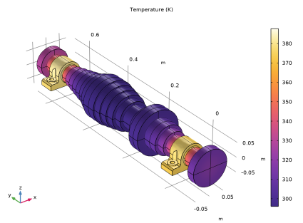
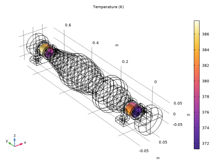
Select the Manual color range checkbox.
4
Set the Maximum value to 4E8.
Deformation
1
In the Model Builder window, expand the Volume 1 node, then click Deformation.
2
In the Settings window for Deformation, locate the Scale section.
3
Select the Scale factor checkbox. In the associated text field, type 50.
4
In the Stress (solid) toolbar, click  Plot.
The default temperature plot in the bearing housing and the rotor is shown in Figure 5.
Temperature (ht)
1
In the Model Builder window, under Results click Temperature (ht).
2
In the Temperature (ht) toolbar, click  Plot.
Follow the instructions below to plot the viscous heat dissipation in the lubricant film as shown in Figure 3.
Viscous Heat
1
In the Results toolbar, click  3D Plot Group.
2
In the Settings window for 3D Plot Group, type Viscous Heat in the Label text field.
3
Locate the Plot Settings section. From the View list, choose New view.
Surface 1
1
Right-click Viscous Heat and choose Surface.
2
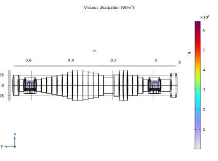
In the Settings window for Surface, click Replace Expression in the upper-right corner of the Expression section. From the menu, choose Component 1 (comp1) > Hydrodynamic Bearing > Journal and bearing properties > Viscous loss > hdb.Qvd - Viscous dissipation - W/m³.
3
Locate the Coloring and Style section. From the Color table list, choose Prism.
4
In the Viscous Heat toolbar, click  Plot.
5
Click the  Go to YZ View button in the Graphics toolbar.
6
Click the  Go to YZ View button in the Graphics toolbar.
7
Click the  Go to YZ View button in the Graphics toolbar.
8
Click the  Zoom Extents button in the Graphics toolbar.
Stress (solid)
Click the  Go to Default View button in the Graphics toolbar.