|
|
|

|
Preload, d
|
||
|
|
|
|
|
|
|
|
|
|
|
|
1
|
|
2
|
In the Select Physics tree, select Structural Mechanics > Rotordynamics > Hydrodynamic Bearing (hdb).
|
|
3
|
Click Add.
|
|
4
|
Click
|
|
5
|
|
6
|
Click
|
|
1
|
|
2
|
|
3
|
Click
|
|
4
|
Browse to the model’s Application Libraries folder and double-click the file hydrodynamic_bearings_comparison_parameters.txt.
|
|
1
|
|
2
|
|
3
|
|
4
|
|
5
|
|
6
|
|
7
|
Click
|
|
1
|
|
2
|
Select the object cyl1 only.
|
|
3
|
|
4
|
|
5
|
|
1
|
|
2
|
|
1
|
|
2
|
|
3
|
|
5
|
Select the Group by continuous tangent checkbox.
|
|
1
|
|
2
|
|
3
|
|
1
|
Repeat above sequence of commands to add more Explicit selections using the information given in the following table:
|
|
2
|
|
1
|
|
2
|
|
3
|
|
1
|
In the Model Builder window, under Component 1 (comp1) > Hydrodynamic Bearing (hdb) click Hydrodynamic Journal Bearing 1.
|
|
2
|
In the Settings window for Hydrodynamic Journal Bearing, type Hydrodynamic Journal Bearing (Cylindrical) in the Label text field.
|
|
3
|
|
4
|
|
5
|
|
6
|
|
7
|
|
8
|
|
9
|
Locate the Fluid Properties section. From the μ list, choose User defined. In the associated text field, type mu.
|
|
10
|
|
11
|
|
12
|
|
1
|
|
2
|
In the Settings window for Hydrodynamic Journal Bearing, type Hydrodynamic Journal Bearing (Elliptical) in the Label text field.
|
|
3
|
|
4
|
|
5
|
|
6
|
|
1
|
|
2
|
In the Settings window for Hydrodynamic Journal Bearing, type Hydrodynamic Journal Bearing (Split halves) in the Label text field.
|
|
3
|
|
4
|
|
5
|
|
6
|
|
7
|
|
1
|
|
2
|
In the Settings window for Hydrodynamic Journal Bearing, type Hydrodynamic Journal Bearing (2-lobe) in the Label text field.
|
|
3
|
|
4
|
|
5
|
|
6
|
|
7
|
|
1
|
|
2
|
In the Settings window for Hydrodynamic Journal Bearing, type Hydrodynamic Journal Bearing (3-lobe LOP) in the Label text field.
|
|
3
|
|
4
|
|
5
|
|
6
|
|
1
|
|
2
|
In the Settings window for Hydrodynamic Journal Bearing, type Hydrodynamic Journal Bearing (3-lobe LBP) in the Label text field.
|
|
3
|
|
1
|
|
2
|
In the Settings window for Hydrodynamic Journal Bearing, type Hydrodynamic Journal Bearing (4-lobe LOP) in the Label text field.
|
|
3
|
|
4
|
|
5
|
|
6
|
|
1
|
|
2
|
In the Settings window for Hydrodynamic Journal Bearing, type Hydrodynamic Journal Bearing (4-lobe LBP) in the Label text field.
|
|
3
|
|
1
|
|
2
|
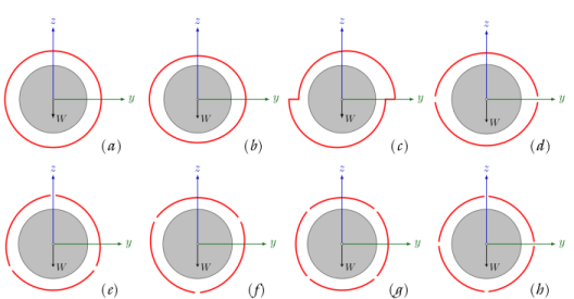
In the Settings window for Bearing Orientation, type Bearing Orientation Hydrodynamic Journal Bearing (3-lobe LOP) in the Label text field.
|
|
3
|
|
4
|
|
1
|
|
2
|
In the Settings window for Bearing Orientation, type Bearing Orientation Hydrodynamic Journal Bearing (3-lobe LBP) in the Label text field.
|
|
3
|
|
4
|
|
1
|
|
2
|
In the Settings window for Bearing Orientation, type Bearing Orientation Hydrodynamic Journal Bearing (4-lobe LOP) in the Label text field.
|
|
3
|
|
4
|
|
1
|
|
2
|
|
3
|
|
1
|
|
2
|
|
3
|
|
4
|
|
5
|
|
1
|
|
2
|
|
3
|
Select the Auxiliary sweep checkbox.
|
|
4
|
Click
|
|
6
|
|
1
|
|
2
|
|
3
|
Click
|
|
4
|
|
5
|
|
6
|
Click OK.
|
|
7
|
|
9
|
Click
|
|
1
|
|
2
|
|
3
|
|
4
|
|
5
|
|
1
|
|
2
|
|
3
|
|
1
|
|
2
|
|
3
|
|
4
|
|
5
|
|
1
|
|
2
|
|
3
|
|
5
|
|
6
|
|
7
|
|
1
|
|
2
|
|
4
|
|
1
|
|
2
|
|
3
|
|
4
|
|
1
|
|
2
|
|
3
|
Locate the y-Axis Data section. In the table, enter the following settings:
|
|
4
|
|
5
|
|
6
|
|
7
|
|
1
|
|
2
|
|
3
|
|
4
|
|
1
|
|
2
|
|
4
|
|
5
|
|
6
|
|
7
|
|
8
|
|
1
|
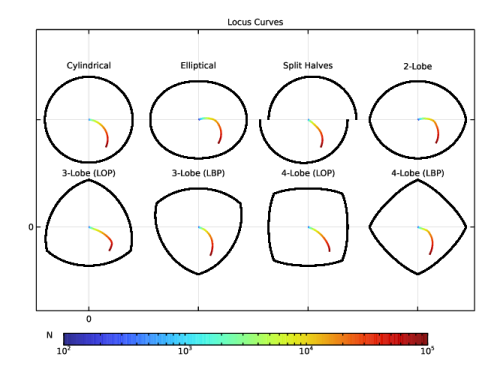
In the Model Builder window, under Results > Locus Curves, Ctrl-click to select Locus Curve (Cylindrical) and Bearing Profile (Cylindrical).
|
|
2
|
Right-click and choose Duplicate.
|
|
1
|
|
2
|
Locate the y-Axis Data section. In the table, enter the following settings:
|
|
3
|
|
1
|
In the Model Builder window, expand the Locus Curve (Elliptical) node, then click Color Expression 1.
|
|
2
|
|
3
|
Clear the Color legend checkbox.
|
|
1
|
|
2
|
|
3
|
|
5
|
|
1
|
In the Model Builder window, under Results > Locus Curves, Ctrl-click to select Locus Curve (Elliptical) and Bearing Profile (Elliptical).
|
|
2
|
|
1
|
|
2
|
|
4
|
|
5
|
|
6
|
|
1
|
|
2
|
|
3
|
|
4
|
Locate the Plot Settings section.
|
|
5
|
|
6
|
|
1
|
|
2
|
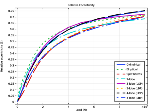
In the Settings window for Global, click Replace Expression in the upper-right corner of the y-Axis Data section. From the menu, choose Component 1 (comp1) > Hydrodynamic Bearing > Hydrodynamic Journal Bearing (Cylindrical) > Eccentricity and attitude angle > hdb.hjb1.ec_rel - Relative eccentricity - 1.
|
|
3
|
Locate the y-Axis Data section. In the table, enter the following settings:
|
|
4
|
Locate the Coloring and Style section. Find the Line style subsection. From the Line list, choose Cycle.
|
|
5
|
|
1
|
|
2
|
|
3
|
|
4
|
|
5
|
|
6
|
|
1
|
|
2
|
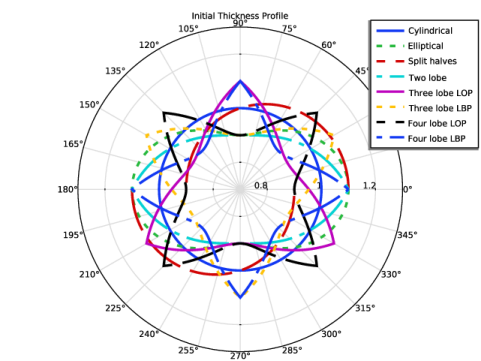
In the Settings window for Polar Plot Group, type Initial Thickness Profile in the Label text field.
|
|
3
|
|
4
|
|
5
|
|
6
|
|
7
|
|
1
|
|
3
|
In the Settings window for Line Graph, click Replace Expression in the upper-right corner of the r-Axis Data section. From the menu, choose Component 1 (comp1) > Hydrodynamic Bearing > Journal and bearing properties > Film thickness and clearance > hdb.hi_rel - Relative film thickness, initial - 1.
|
|
4
|
Locate the r-Axis Data section.
|
|
5
|
|
6
|
|
7
|
|
8
|
Click to expand the Coloring and Style section. Find the Line style subsection. From the Line list, choose Cycle.
|
|
9
|
|
10
|
|
11
|
|
12
|
Select the Label checkbox.
|
|
13
|
|
1
|
|
2
|
|
3
|
|
5
|
|
1
|
|
2
|
|
1
|
|
2
|
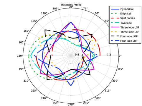
In the Settings window for Polar Plot Group, type Current Thickness Profile in the Label text field.
|
|
3
|
|
4
|
|
1
|
Edit the existing Line Graph nodes under Polar: Current Thickness Profile using the information given in the following table:
|
|
2
|
In the Model Builder window, expand the Current Thickness Profile node, then click Results > Current Thickness Profile.
|
|
3
|
|
4
|
|
5
|
|
6
|
|
7
|
|
8
|
|
1
|
|
2
|
Go to the Result Templates window.
|
|
3
|
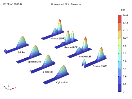
In the tree, select Study 1/Solution 1 (sol1) > Hydrodynamic Bearing > Unwrapped Plots (hjb1), Study 1/Solution 1 (sol1) > Hydrodynamic Bearing > Unwrapped Plots (hjb2), Study 1/Solution 1 (sol1) > Hydrodynamic Bearing > Unwrapped Plots (hjb3), Study 1/Solution 1 (sol1) > Hydrodynamic Bearing > Unwrapped Plots (hjb4), Study 1/Solution 1 (sol1) > Hydrodynamic Bearing > Unwrapped Plots (hjb5), Study 1/Solution 1 (sol1) > Hydrodynamic Bearing > Unwrapped Plots (hjb6), Study 1/Solution 1 (sol1) > Hydrodynamic Bearing > Unwrapped Plots (hjb7), and Study 1/Solution 1 (sol1) > Hydrodynamic Bearing > Unwrapped Plots (hjb8).
|
|
4
|
Click the Add Result Template button in the window toolbar.
|
|
5
|
|
1
|
|
2
|
|
3
|
|
4
|
|
5
|
|
6
|
|
7
|
|
8
|
|
1
|
|
2
|
|
1
|
|
2
|
|
3
|
|
4
|
|
5
|
|
6
|
|
7
|
|
1
|
|
2
|
|
3
|
|
5
|
|
6
|
|
7
|
|
8
|
|
9
|
|
1
|
|
2
|
|
3
|
|
4
|
|
5
|
|
6
|
|
7
|
|
8
|
|
9
|
|
1
|
|
2
|
|
3
|
|
1
|
|
2
|
|
3
|
|
1
|
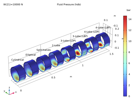
In the Model Builder window, under Results > Unwrapped Velocity, Ctrl-click to select Pressure (Cylindrical) and Velocity (Cylindrical).
|
|
2
|
Right-click and choose Duplicate.
|
|
1
|
|
2
|
|
3
|
|
4
|
|
5
|
|
1
|
|
2
|
|
3
|
|
4
|
|
5
|
|
6
|
|
1
|
|
2
|
|
3
|
|
5
|
|
6
|
|
7
|
|
8
|