|
|
|
|
mPa⋅s
|
||
|
GPa-1
|
||
|
kg/m3
|
|
•
|
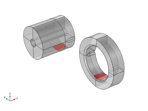
Use the Solid Mechanics interface along with the Hydrodynamic Bearing interface to set up the elastohydrodynamic model.
|
|
•
|
This model shows how to set up a manual coupling between the Solid Mechanics and Hydrodynamic Bearing interfaces. As an alternative approach, the built-in multiphysics coupling Solid-Bearing Coupling automatically couples the Solid Mechanics and Hydrodynamic Bearing interface. Note that the built-in coupling uses an approximated displacement field for the journal and bearing displacements, which makes it incapable to represent local deformations which are important for this model.
|
|
1
|
|
2
|
In the Select Physics tree, select Structural Mechanics > Solid Mechanics (solid) and Structural Mechanics > Rotordynamics > Hydrodynamic Bearing (hdb).
|
|
3
|
Click Add.
|
|
4
|
Click
|
|
5
|
|
6
|
Click
|
|
1
|
|
2
|
|
1
|
|
2
|
|
3
|
|
4
|
|
5
|
|
1
|
|
2
|
|
3
|
|
4
|
|
5
|
|
1
|
|
2
|
|
3
|
Click
|
|
4
|
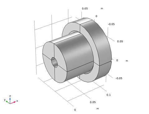
Browse to the model’s Application Libraries folder and double-click the file elastohydrodynamic_journal_bearing.mphbin.
|
|
5
|
Click
|
|
1
|
|
2
|
|
3
|
|
4
|
Select the Create imprints checkbox.
|
|
5
|
|
1
|
|
2
|
|
3
|
|
4
|
|
5
|
Click
|
|
6
|
|
7
|
Click OK.
|
|
1
|
|
2
|
|
3
|
|
4
|
Select the Group by continuous tangent checkbox.
|
|
5
|
Click
|
|
6
|
|
7
|
Click OK.
|
|
1
|
|
2
|
|
3
|
|
4
|
Select the Group by continuous tangent checkbox.
|
|
5
|
Click
|
|
6
|
|
7
|
Click OK.
|
|
1
|
|
2
|
|
3
|
|
4
|
Click
|
|
5
|
|
6
|
Click OK.
|
|
1
|
|
2
|
|
3
|
|
4
|
|
5
|
|
6
|
Click
|
|
7
|
|
8
|
Click OK.
|
|
1
|
|
2
|
|
3
|
|
4
|
Select the Group by continuous tangent checkbox.
|
|
5
|
Click
|
|
6
|
|
7
|
Click OK.
|
|
1
|
|
2
|
|
3
|
|
4
|
Select the Group by continuous tangent checkbox.
|
|
5
|
Click
|
|
6
|
|
7
|
Click OK.
|
|
1
|
|
2
|
|
3
|
|
4
|
Click
|
|
5
|
|
6
|
Click OK.
|
|
1
|
|
2
|
Go to the Add Material window.
|
|
3
|
|
4
|
Click the Add to Component button in the window toolbar.
|
|
5
|
|
1
|
In the Model Builder window, under Component 1 (comp1) right-click Materials and choose Blank Material.
|
|
2
|
|
3
|
Locate the Geometric Entity Selection section. From the Geometric entity level list, choose Boundary.
|
|
4
|
|
5
|
Locate the Material Contents section. In the table, enter the following settings:
|
|
1
|
In the Model Builder window, under Component 1 (comp1) > Solid Mechanics (solid) click Continuity 1.
|
|
2
|
|
3
|
Select the Disconnect pair checkbox.
|
|
1
|
|
2
|
|
3
|
|
1
|
|
2
|
|
3
|
|
1
|
|
2
|
|
3
|
|
4
|
|
5
|
Select the Constrain rotation around x-axis checkbox.
|
|
1
|
|
2
|
In the Settings window for Boundary Load, type Boundary Load (Supply Pressure) in the Label text field.
|
|
3
|
|
4
|
|
5
|
|
1
|
|
2
|
In the Settings window for Boundary Load, type Boundary Load (Fluid Load, Journal) in the Label text field.
|
|
3
|
Locate the Boundary Selection section. From the Selection list, choose Hydrodynamic Bearing (Journal).
|
|
4
|
|
1
|
|
2
|
In the Settings window for Boundary Load, type Boundary Load (Fluid Load, Bearing) in the Label text field.
|
|
3
|
Locate the Boundary Selection section. From the Selection list, choose Hydrodynamic Bearing (Bearing).
|
|
4
|
|
1
|
|
2
|
In the Settings window for Boundary Load, type Boundary Load (Bearing Load) in the Label text field.
|
|
3
|
|
4
|
|
5
|
|
1
|
|
2
|
|
3
|
|
1
|
In the Model Builder window, under Component 1 (comp1) > Hydrodynamic Bearing (hdb) click Hydrodynamic Journal Bearing 1.
|
|
2
|
|
3
|
|
5
|
|
6
|
|
7
|
|
1
|
|
2
|
|
3
|
|
1
|
|
2
|
|
1
|
|
2
|
|
3
|
|
4
|
|
5
|
|
1
|
|
2
|
|
3
|
|
5
|
|
1
|
|
2
|
|
3
|
|
4
|
Locate the Second Entity Group section. From the Selection list, choose Hydrodynamic Bearing (Bearing).
|
|
1
|
|
1
|
|
3
|
|
4
|
|
1
|
|
3
|
|
4
|
|
5
|
|
6
|
|
7
|
|
1
|
|
2
|
|
3
|
|
1
|
|
2
|
|
1
|
|
2
|
|
3
|
Clear the Generate default plots checkbox.
|
|
1
|
|
2
|
|
3
|
Select the Auxiliary sweep checkbox.
|
|
4
|
Click
|
|
1
|
|
2
|
|
3
|
Right-click Study 1 > Solver Configurations > Solution 1 (sol1) > Stationary Solver 1 and choose Fully Coupled.
|
|
4
|
|
1
|
|
2
|
|
3
|
|
4
|
Click
|
|
5
|
|
6
|
|
7
|
Click OK.
|
|
8
|
|
10
|
Click
|
|
11
|
|
12
|
|
13
|
Click OK.
|
|
14
|
|
16
|
Click
|
|
17
|
|
18
|
|
19
|
Click OK.
|
|
20
|
|
22
|
Click
|
|
1
|
|
2
|
|
3
|
|
1
|
|
2
|
|
3
|
|
4
|
|
5
|
|
6
|
|
1
|
|
2
|
|
3
|
|
4
|
|
1
|
|
2
|
|
3
|
|
4
|
|
5
|
|
1
|
|
2
|
|
3
|
|
1
|
|
2
|
|
3
|
Click
|
|
4
|
|
5
|
Click OK.
|
|
6
|
|
1
|
|
2
|
|
3
|
|
4
|
|
5
|
|
6
|
|
7
|
|
1
|
|
2
|
|
3
|
|
1
|
|
2
|
|
3
|
Click
|
|
4
|
|
6
|
|
1
|
|
2
|
|
3
|
Select the Use the plot’s color checkbox.
|
|
1
|
|
2
|
|
3
|
|
1
|
|
2
|
|
3
|
Click
|
|
5
|
|
1
|
|
2
|
|
3
|
|
4
|
|
5
|
|
6
|
|
7
|
|
8
|
|
1
|
|
2
|
|
3
|
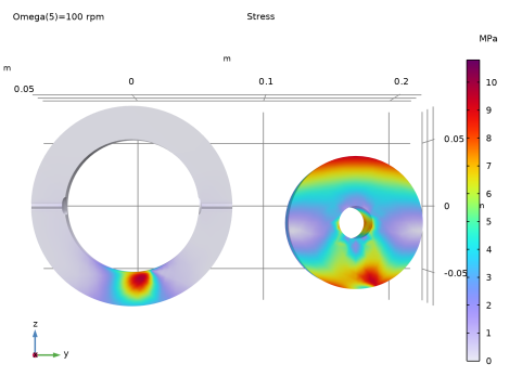
Click Replace Expression in the upper-right corner of the Expression section. From the menu, choose Component 1 (comp1) > Solid Mechanics > Stress > solid.misesGp - von Mises stress - N/m².
|
|
4
|
|
1
|
|
2
|
|
3
|
|
1
|
|
2
|
|
3
|
|
1
|
|
2
|
|
3
|
Click
|
|
5
|
|
1
|
In the Model Builder window, under Component 1 (comp1) > Hydrodynamic Bearing (hdb) right-click Hydrodynamic Journal Bearing 1 and choose Duplicate.
|
|
2
|
|
3
|
|
4
|
|
1
|
In the Model Builder window, expand the Hydrodynamic Journal Bearing 2 node, then click Moving Foundation 1.
|
|
2
|
|
3
|
|
1
|
|
2
|
|
3
|
Select the Modify model configuration for study step checkbox.
|
|
4
|
In the tree, select Component 1 (comp1) > Hydrodynamic Bearing (hdb) > Hydrodynamic Journal Bearing 2.
|
|
5
|
Click
|
|
1
|
|
2
|
Go to the Add Study window.
|
|
3
|
|
4
|
Click the Add Study button in the window toolbar.
|
|
5
|
|
1
|
|
2
|
Clear the Generate default plots checkbox.
|
|
1
|
|
2
|
|
3
|
Select the Modify model configuration for study step checkbox.
|
|
4
|
|
5
|
Click
|
|
6
|
|
7
|
Click
|
|
9
|
|
1
|
|
2
|
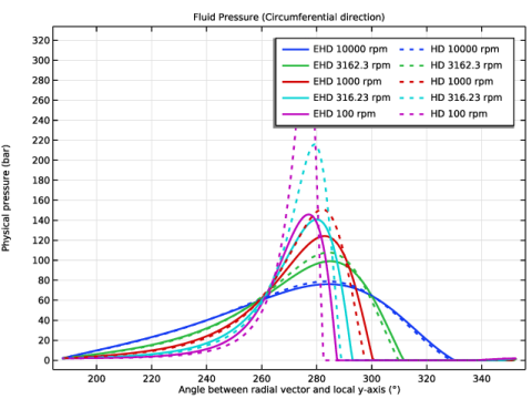
In the Settings window for 1D Plot Group, type Fluid Pressure (Circumferential direction) in the Label text field.
|
|
3
|
|
4
|
|
5
|
|
1
|
|
2
|
|
4
|
|
5
|
|
6
|
|
7
|
|
8
|
|
9
|
|
1
|
|
2
|
|
3
|
|
4
|
Locate the Coloring and Style section. Find the Line style subsection. From the Line list, choose Dotted.
|
|
5
|
|
1
|
|
2
|
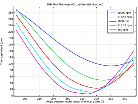
In the Settings window for 1D Plot Group, type EHD Film Thickness (Circumferential direction) in the Label text field.
|
|
3
|
|
1
|
|
3
|
|
4
|
|
5
|
|
6
|
|
7
|
|
8
|
|
9
|
|
10
|
|
1
|
|
2
|
Go to the Result Templates window.
|
|
3
|
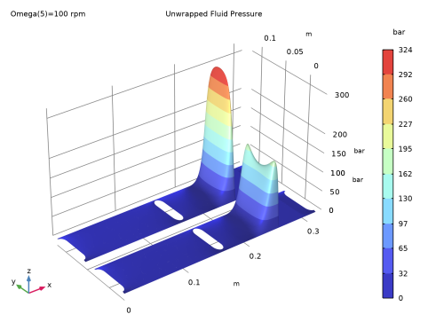
In the tree, select Study 1/Solution 1 (sol1) > Hydrodynamic Bearing > Unwrapped Plots (hjb1) > Unwrapped Fluid Pressure (hjb1).
|
|
4
|
Click the Add Result Template button in the window toolbar.
|
|
5
|
In the tree, select Study 2/Solution 2 (sol2) > Hydrodynamic Bearing > Unwrapped Plots (hjb2) > Unwrapped Fluid Pressure (hjb2).
|
|
6
|
Click the Add Result Template button in the window toolbar.
|
|
7
|
|
1
|
|
2
|
|
3
|
|
4
|
|
5
|
|
1
|
|
2
|
|
3
|
|
1
|
|
2
|
|
3
|
|
4
|
|
5
|
|
6
|
|
7
|
|
1
|
|
2
|
|
1
|
|
2
|
|
3
|
|
4
|
|
5
|