PDF

Rotors Connected by a Spline Coupling
Introduction
This example demonstrates a method for coupling two rotors connected by a spline coupling. An eigenfrequency analysis is performed at different rotor speeds, and the results are compared with those obtained in Ref. 1.
Model Definition
The model consists an assembly of two rotors connected through a spline coupling. The rotor configuration is visualized in Figure 1. The first rotor, spanning from point A to C, has a fixed support at point A and is equipped with a disk at point B. The second rotor, spanning from point C to F, is simply supported at point D and F. A pulley is mounted at point E. The rotors are connected through point C. It is assumed that only translational motion is coupled between the rotors through the coupling, while the rotations are uncoupled.
Figure 1: Rotor geometry.
The disk mounted on the cantilevered rotor has both mass and moment of inertia. The coupling has only mass with negligible moment of inertia. In addition, the pulley mounted on the simply supported rotor has only mass but negligible moment of inertia.
The properties of the shaft are summarized in the Table 1.
The properties of the mountings on the shafts are given in the Table 2.
Results and Discussion
Figure 2 below shows the whirl plots for the second forward and backward mode at
50,000 rpm. The discontinuity in the rotational degrees of freedom is clearly visible at the coupling location. The undeformed geometry of the rotor is also shown below the whirl plots.
Figure 2: Whirl plots of forward and backward whirl at 50,000 rpm.
The gyroscopic effect in the rotor stiffens the forward modes and softens the backward modes. This phenomenon is illustrated in the Campbell diagram shown in Figure 3. A comparison of the critical speeds (in rpm) with those of Ref. 1 is given in Table 3.
It is clear that the second mode is relatively unaffected by the gyroscopic effect. However, the fourth mode is very strongly influenced by the gyroscopic effect.
Figure 3: Campbell diagram.
Reference
1. W.J. Chen and E.J. Gunter, Introduction to the Dynamics of Rotor-Bearing Systems, Example 5.3, pp. 186–189, Trafford Publishing, 2007.
Application Library path: Rotordynamics_Module/Verification_Examples/coupled_rotors
Modeling Instructions
From the File menu, choose New.
New
In the New window, click  Model Wizard.
Model Wizard
1
In the Model Wizard window, click  3D.
2
In the Select Physics tree, select Structural Mechanics > Rotordynamics > Beam Rotor (rotbm).
3
Click Add.
4
Click  Study.
5
In the Select Study tree, select General Studies > Eigenfrequency.
6
Global Definitions
Parameters 1
1
In the Model Builder window, under Global Definitions click Parameters 1.
2
In the Settings window for Parameters, locate the Parameters section.
3
Geometry 1
Polygon 1 (pol1)
1
In the Geometry toolbar, click  More Primitives and choose Polygon.
2
In the Settings window for Polygon, locate the Coordinates section.
3
From the Data source list, choose Vectors.
4
In the x text field, type 0 x_disk x_coupling x_support1 x_pulley x_support2.
5
In the y text field, type 0.
6
In the z text field, type 0.
Beam Rotor (rotbm)
1
In the Model Builder window, under Component 1 (comp1) click Beam Rotor (rotbm).
2
In the Settings window for Beam Rotor, locate the Rotor Speed section.
3
Set the Linear Elastic Material to use the Young’s modulus and shear modulus as the elastic properties.
Linear Elastic Material 1
1
In the Model Builder window, under Component 1 (comp1) > Beam Rotor (rotbm) click Linear Elastic Material 1.
2
In the Settings window for Linear Elastic Material, locate the Linear Elastic Material section.
3
From the Specify list, choose Young’s modulus and shear modulus.
Materials
Material 1 (mat1)
1
In the Model Builder window, under Component 1 (comp1) right-click Materials and choose Blank Material.
2
In the Settings window for Material, locate the Material Contents section.
3
Beam Rotor (rotbm)
Rotor Cross Section 1
1
In the Model Builder window, under Component 1 (comp1) > Beam Rotor (rotbm) click Rotor Cross Section 1.
2
In the Settings window for Rotor Cross Section, locate the Cross-Section Definition section.
3
In the do text field, type d_shaft.
Disk 1
1
In the Physics toolbar, click  Points and choose Disk.
2
3
In the Settings window for Disk, locate the Disk Properties section.
4
In the m text field, type m_disk.
5
In the Ip text field, type Ip_disk.
6
In the Id text field, type Id_disk.
Disk: Coupling
1
In the Physics toolbar, click  Points and choose Disk.
2
In the Settings window for Disk, type Disk: Coupling in the Label text field.
3
4
Locate the Disk Properties section. In the m text field, type m_coupling.
Disk: Pulley
1
Right-click Disk: Coupling and choose Duplicate.
2
In the Settings window for Disk, type Disk: Pulley in the Label text field.
3
Locate the Point Selection section. Click  Clear Selection.
4
5
Locate the Disk Properties section. In the m text field, type m_pulley.
Journal Bearing: Fixed
1
In the Physics toolbar, click  Points and choose Journal Bearing.
2
In the Settings window for Journal Bearing, type Journal Bearing: Fixed in the Label text field.
3
Journal Bearing: Pinned
1
Right-click Journal Bearing: Fixed and choose Duplicate.
2
In the Settings window for Journal Bearing, type Journal Bearing: Pinned in the Label text field.
3
Locate the Point Selection section. Click  Clear Selection.
4
5
Locate the Bearing Properties section. Clear the Constrain bending rotation checkbox.
Rotor Coupling 1
1
In the Physics toolbar, click  Points and choose Rotor Coupling.
2
Study 1
Add a parametric step to sweep the rpm from 0 to 50000 in steps of 2000.
Parametric Sweep
1
In the Study toolbar, click  Parametric Sweep.
2
In the Settings window for Parametric Sweep, locate the Study Settings section.
3
4
Step 1: Eigenfrequency
Now, increase the number of desired eigenfrequencies, and activate mode following for continuous tracking of the eigenfrequencies over the swept interval.
1
In the Model Builder window, click Step 1: Eigenfrequency.
2
In the Settings window for Eigenfrequency, locate the Study Settings section.
3
Select the Desired number of eigenfrequencies checkbox. In the associated text field, type 10.
4
Click to expand the Filtering and Sorting section. Find the Sorting subsection. Select the Mode following checkbox.
5
In the Study toolbar, click  Compute.
Results
Whirl (rotbm)
Follow the steps below to generate the whirl plots shown in Figure 2.
1
In the Settings window for 3D Plot Group, locate the Data section.
2
From the Eigenfrequency (Hz) list, choose 311.96.
Whirl 1
1
In the Model Builder window, expand the Whirl (rotbm) node, then click Whirl 1.
2
In the Settings window for Whirl, locate the Coloring and Style section.
3
In the Number of planes text field, type 6.
4
In the Whirl (rotbm) toolbar, click  Plot.
5
Click the  Go to Default View button in the Graphics toolbar.
6
Click the  Zoom Extents button in the Graphics toolbar.
Now, create a Campbell diagram. This can be done by following the instructions below.
Result Templates
1
In the Results toolbar, click  Result Templates to open the Result Templates window.
2
Go to the Result Templates window.
3
In the tree, select Study 1/Parametric Solutions 1 (sol2) > Beam Rotor > Campbell Diagram (rotbm).
4
Click the Add Result Template button in the window toolbar.
5
In the Results toolbar, click  Result Templates to close the Result Templates window.
Results
Campbell Diagram (rotbm)
1
In the Settings window for 1D Plot Group, locate the Data section.
2
From the Eigenfrequency selection list, choose Manual.
3
In the Eigenfrequency indices (1-10) text field, type range(1,1,8).
4
Locate the Axis section. Select the Manual axis limits checkbox.
5
In the y maximum text field, type 1000.
6
In the y minimum text field, type -20.
7
In the Model Builder window, expand the Campbell Diagram (rotbm) node.
Natural Frequency
1
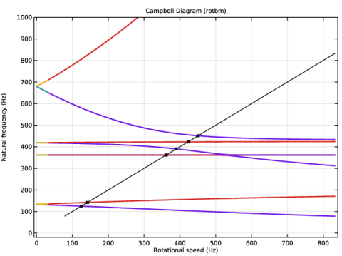
In the Model Builder window, expand the Campbell Diagram (rotbm) node, then click Natural Frequency.
2
In the Settings window for Global, locate the y-Axis Data section.
3
4
In the Campbell Diagram (rotbm) toolbar, click  Plot.
Follow the steps below to generate a mode shape plot.
Mode Shape
1
In the Results toolbar, click  3D Plot Group.
2
In the Settings window for 3D Plot Group, type Mode Shape in the Label text field.
3
Locate the Data section. From the Dataset list, choose Study 1/Parametric Solutions 1 (sol2).
4
From the Parameter value (Ow (rpm)) list, choose 8000.
5
From the Eigenfrequency (Hz) list, choose 420.35.
Line 1
1
Right-click Mode Shape and choose Line.
2
In the Settings window for Line, locate the Coloring and Style section.
3
From the Line type list, choose Tube.
4
In the Tube radius expression text field, type rotbm.re.
5
From the Color table list, choose AuroraAustralis.
6
Clear the Color legend checkbox.
Deformation 1
1
Right-click Line 1 and choose Deformation.
2
In the Settings window for Deformation, locate the Scale section.
3
Select the Scale factor checkbox. In the associated text field, type 0.3.
4
Click the  Go to XY View button in the Graphics toolbar.
5
In the Mode Shape toolbar, click  Plot.
6
Click the  Zoom Extents button in the Graphics toolbar.