PDF

Vdara® Caustic Surface
Introduction
When the Vdara® hotel first opened in Las Vegas, visitors relaxing by the pool would experience intense periods of heat at certain times of the day and at certain times of the year. This intense heat was caused by the reflection of solar radiation from the curved, reflective surface on the South-facing side of the hotel. This model shows how a caustic surface is generated in the pool area around the time and date the problems were first reported.
Note: This application also requires the CAD Import Module.
Figure 1 below shows a small area of the CityCenter® complex which is the subject of this model. The concave surfaces of the Vdara® hotel are illuminated by sunlight, indicated by red arrows, at certain times of the day. The direction of the reflected rays depends on the direction of the incident solar radiation and the surface normal of the hotel.
Figure 1: A solar flux incident on the concave surface of the Vdara® hotel is reflected down to the pool area beneath.
The Geometrical Optics interface can compute the intensity along individual ray paths by computing the principal radii of curvature of the associated wavefronts. When plane waves are reflected by the surface of the hotel, these principal radii of curvature are changed. When the rays are reflected by a concave surface, the radius of curvature decreases in magnitude thereafter and eventually approaches zero. A continuous set of points at which either principal radius of curvature equals zero is called a caustic surface. In lens systems, the caustic surface often demarcates an envelope of rays. In the limit of geometrical optics, the ray intensity is infinite on a caustic surface. Practically, this corresponds to locations where the incident heat flux is extremely high, which can cause severe burns.
Model Definition
The model geometry includes the Vdara® hotel and several nearby buildings in the CityCenter® complex.
Figure 2: Imported CAD geometry of a section of the CityCenter® complex. The Vdara® hotel is shown at the top.
In order to avoid having to trace rays from the sun onto the surface of the hotel, a special boundary condition called the Illuminated Surface is employed. This boundary condition allows rays to be released from the surface of the hotel directly, significantly reducing the simulation time. The direction at which the rays are released from the surface of the hotel depends on the incoming ray direction vector n and the outward surface normal ns, according to the formula
The principal radii of curvature of the released rays are also computed based on the radii of curvature of the incident wavefront and the curvature of the surface of the hotel. More details can be found in the Ray Optics Module User’s Guide.
When the rays arrive at the swimming pool area, the intensity value of each ray is projected onto the surface mesh. This allows for more convenient visualization of the intersection of the caustic surface with the boundary. The Accumulator feature is used to accomplish this by implementing the following equation:
where Rj is the value of an arbitrary source term for the jth incident ray, qj is the position of the jth ray when it strikes the pool area, and rb is the value of the accumulated variable on a given boundary mesh element. Any expression for the source term Rj may be defined; for this example, Rj=log(Ij) is used, where Ij is the intensity of the jth ray. The sum is taken over all rays that reach a given boundary element. The logarithm is used to better visualize changes in the order of magnitude of the ray intensity.
The selections for the boundary conditions are shown below. The curved, reflective surfaces of the hotel that face the sun are shown in orange. The other surfaces of the hotel are shown in gold. The pool and the surrounding area are shown in blue.
Figure 3: Close-up view of the Vdara® hotel.
Results and Discussion
The trajectories of the rays can be seen in Figure 4. The rays begin to cross each other after they reflect off the surface of the hotel. The color represents the intensity, which becomes very high at specific locations, indicated by the green and red coloring.
Figure 4: Ray trajectories reflecting off the Vdara® hotel in September at 11:45 am. The arrows indicate the direction vector of the solar radiation.
The projection of the high-intensity regions onto the swimming pool area is plotted in Figure 5. As expected, for this specific time of month and day, there is a clearly visible caustic surface cutting directly across the pool yard.
Figure 5: Plot of the log of the intensity projected onto the swimming pool area. There is a region of very high intensity right across the swimming pool.
Reference
1. M. Vollmer and K-P. Möllmann, “Caustic effects due to sunlight reflections from skyscrapers: simulations and experiments,” Eur. J. Phys., vol. 33, pp. 1429–1455, 2012.
Application Library path: Ray_Optics_Module/Solar_Radiation/vdara_caustic_surface
Modeling Instructions
From the File menu, choose New.
New
In the New window, click  Model Wizard.
Model Wizard
1
In the Model Wizard window, click  3D.
2
In the Select Physics tree, select Optics > Ray Optics > Geometrical Optics (gop).
3
Click Add.
4
Click  Study.
5
In the Select Study tree, select Preset Studies for Selected Physics Interfaces > Ray Tracing.
6
Geometry 1
1
In the Model Builder window, under Component 1 (comp1) click Geometry 1.
2
In the Settings window for Geometry, locate the Units section.
3
From the Length unit list, choose km.
4
This example uses an imported CAD geometry. Check that CAD kernel is selected from the Geometry representation list.
Import 1 (imp1)
1
In the Geometry toolbar, click  Import.
2
In the Settings window for Import, locate the Source section.
3
Click  Browse.
4
5
Click  Import.
Compare the imported geometry to Figure 2.
Disable the analysis of the geometry as the remaining small geometric details can be kept.
6
In the Model Builder window, click Geometry 1.
7
In the Settings window for Geometry, locate the Cleanup section.
8
Clear the Automatic detection of small details checkbox.
9
In the Geometry toolbar, click  Build All.
Definitions
Create a Box selection that contains all of the surfaces of the hotel.
Hotel Surfaces
1
In the Definitions toolbar, click  Box.
2
In the Settings window for Box, type Hotel Surfaces in the Label text field.
3
Locate the Output Entities section. From the Include entity if list, choose Entity inside box.
4
Locate the Geometric Entity Level section. From the Level list, choose Boundary.
5
Locate the Box Limits section. In the x minimum text field, type 0.475.
6
In the x maximum text field, type 0.52.
7
In the y minimum text field, type 0.38.
8
In the y maximum text field, type 0.5.
9
In the z minimum text field, type 0.01.
10
In the z maximum text field, type 0.2.
All of the surfaces of the hotel should be selected, including the orange and gold surfaces in Figure 3.
Geometrical Optics (gop)
1
In the Model Builder window, under Component 1 (comp1) click Geometrical Optics (gop).
2
In the Settings window for Geometrical Optics, locate the Domain Selection section.
3
Click  Clear Selection.
4
Locate the Ray Release and Propagation section. In the Maximum number of secondary rays text field, type 0.
5
Locate the Intensity Computation section. From the Intensity computation list, choose Compute intensity.
Selecting the Store ray status data checkbox causes a variable for the final ray status available for postprocessing; this will be used to filter rays so that only the rays that reach the pool are viewed.
6
Locate the Additional Variables section. Select the Store ray status data checkbox.
Illuminated Surface 1
1
In the Physics toolbar, click  Boundaries and choose Illuminated Surface.
2
3
In the Settings window for Illuminated Surface, locate the Initial Position section.
4
From the Initial position list, choose Density.
5
In the N text field, type 50000.
6
Locate the Ray Direction Vector section. From the Incident ray direction vector list, choose Solar radiation.
7
From the Location defined by list, choose City.
8
9
Wall 1
1
In the Physics toolbar, click  Boundaries and choose Wall.
2
Accumulator 1
1
In the Physics toolbar, click  Attributes and choose Accumulator.
2
In the Settings window for Accumulator, locate the Accumulator Settings section.
3
From the Accumulate over list, choose Rays in boundary elements.
4
In the R text field, type gop.logI.
The Source text field will turn yellow and a tooltip warning will appear, indicating that the deduced unit does not match the expected unit. Fix this by specifying the dependent variable quantity.
5
Locate the Units section. Click  Custom Unit.
6
In the Dependent variable quantity table, enter the following settings:
Wall 2
1
In the Physics toolbar, click  Boundaries and choose Wall.
The second Wall condition allows rays to be reflected multiple times at different surfaces of the building.
2
In the Settings window for Wall, locate the Boundary Selection section.
3
From the Selection list, choose Hotel Surfaces.
4
Locate the Wall Condition section. From the Wall condition list, choose Specular reflection.
Mesh 1
1
In the Model Builder window, under Component 1 (comp1) click Mesh 1.
2
In the Settings window for Mesh, locate the Physics-Controlled Mesh section.
3
From the Element size list, choose Extremely fine.
4
Click  Build All.
Study 1
Step 1: Ray Tracing
1
In the Model Builder window, under Study 1 click Step 1: Ray Tracing.
2
In the Settings window for Ray Tracing, locate the Study Settings section.
3
From the Time-step specification list, choose Specify maximum path length.
4
Click  Range.
5
In the Range dialog, type 10 in the Step text field.
6
In the Stop text field, type 200.
7
Click Replace.
8
In the Study toolbar, click  Compute.
Results
Ray Trajectories (gop)
1
In the Settings window for 3D Plot Group, click to expand the Title section.
2
From the Title type list, choose Manual.
3
In the Title text area, type Reflected Rays and Ambient Solar Radiation.
Grid 3D 1
The default plot shows the paths of the reflected rays. The direction of the incident solar radiation is also shown as a vector field. First, adjust the Grid 3D dataset so that the vectors are closer together.
1
In the Model Builder window, expand the Results > Datasets node, then click Grid 3D 1.
2
In the Settings window for Grid 3D, locate the Parameter Bounds section.
3
Find the First parameter subsection. In the Minimum text field, type 0.4.
4
In the Maximum text field, type 0.48.
5
Find the Second parameter subsection. In the Minimum text field, type 0.4.
6
In the Maximum text field, type 0.48.
7
Find the Third parameter subsection. In the Minimum text field, type 0.05.
8
In the Maximum text field, type 0.15.
Ray Trajectories (gop)
Now resume editing the Ray Trajectories plot.
In the Model Builder window, expand the Results > Ray Trajectories (gop) node.
Color Expression 1
1
In the Model Builder window, expand the Results > Ray Trajectories (gop) > Ray Trajectories 1 node, then click Color Expression 1.
2
In the Settings window for Color Expression, click Replace Expression in the upper-right corner of the Expression section. From the menu, choose Component 1 (comp1) > Geometrical Optics > Intensity and polarization > gop.logI - Log of intensity - 1.
Filter 1
Plot only the rays with final status gop.fs==2. This is true for all rays that have hit a Wall with the Freeze condition; that is, all rays that have reached the pool. Filtering the rays makes the solution easier to visualize.
1
In the Model Builder window, click Filter 1.
2
In the Settings window for Filter, locate the Ray Selection section.
3
From the Rays to include list, choose Logical expression.
4
In the Logical expression for inclusion text field, type gop.fs==2.
Ray Trajectories (gop)
Add a Surface plot to the building and poolside to make them appear solid.
Surface 1
1
In the Model Builder window, right-click Ray Trajectories (gop) and choose Surface.
2
In the Settings window for Surface, locate the Coloring and Style section.
3
From the Coloring list, choose Uniform.
4
From the Color list, choose Gray.
5
In the Ray Trajectories (gop) toolbar, click  Plot.
6
Click the  Go to Default View button in the Graphics toolbar. Compare the resulting plot to Figure 4.
Caustic Surface in Pool Area
1
In the Results toolbar, click  3D Plot Group.
2
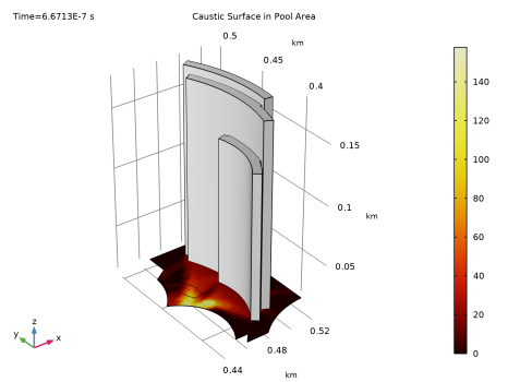
In the Settings window for 3D Plot Group, type Caustic Surface in Pool Area in the Label text field.
3
Locate the Title section. From the Title type list, choose Manual.
4
In the Title text area, type Caustic Surface in Pool Area.
Surface 1
1
Right-click Caustic Surface in Pool Area and choose Surface.
2
In the Settings window for Surface, click Replace Expression in the upper-right corner of the Expression section. From the menu, choose Component 1 (comp1) > Geometrical Optics > Accumulated variables > Accumulated variable comp1.gop.wall1.bacc1.rpb > gop.wall1.bacc1.rpb - Accumulated variable rpb - 1/m².
3
Click to expand the Quality section. From the Evaluation settings list, choose Manual.
4
From the Smoothing list, choose Everywhere.
5
From the Resolution list, choose No refinement.
6
Locate the Coloring and Style section. From the Color table list, choose ThermalDark.
Create another Surface plot to display the surfaces of the hotel.
Caustic Surface in Pool Area
In the Model Builder window, click Caustic Surface in Pool Area.
Surface 2
1
In the Caustic Surface in Pool Area toolbar, click  Surface.
2
In the Settings window for Surface, click to expand the Title section.
3
From the Title type list, choose None.
4
Locate the Coloring and Style section. From the Coloring list, choose Uniform.
5
From the Color list, choose Gray.
Selection 1
1
Right-click Surface 2 and choose Selection.
2
In the Settings window for Selection, locate the Selection section.
3
From the Selection list, choose Hotel Surfaces.
4
In the Caustic Surface in Pool Area toolbar, click  Plot.
5
Click the  Go to Default View button in the Graphics toolbar. Compare the resulting plot to Figure 5.