 | 
|
|
|
|
|
1
|
|
2
|
|
3
|
Click Add.
|
|
4
|
Click
|
|
5
|
|
6
|
Click
|
|
1
|
|
2
|
|
3
|
|
1
|
|
2
|
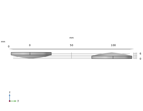
In the Part Libraries window, select Ray Optics Module > 3D > Spherical Lenses > spherical_plano_convex_lens_3d in the tree.
|
|
3
|
Click
|
|
4
|
In the Select Part Variant dialog, select Specify effective focal length and center thickness in the Select part variant list.
|
|
5
|
Click OK.
|
|
1
|
In the Model Builder window, under Component 1 (comp1) > Geometry 1 right-click Spherical Plano-Convex Lens 3D 1 (pi1) and choose Duplicate.
|
|
2
|
|
4
|
Locate the Position and Orientation of Output section. Find the Displacement subsection. In the ywi text field, type 100[mm].
|
|
5
|
|
6
|
Click
|
|
1
|
|
2
|
|
1
|
|
2
|
|
3
|
|
4
|
|
1
|
In the Model Builder window, under Component 1 (comp1) > Geometrical Optics (gop) click Material Discontinuity 1.
|
|
2
|
|
3
|
|
1
|
|
2
|
|
3
|
|
4
|
|
5
|
|
6
|
|
7
|
|
8
|
|
1
|
|
2
|
|
3
|
|
1
|
|
2
|
|
3
|
|
4
|
Click
|
|
1
|
|
2
|
|
3
|
|
4
|
|
1
|
|
2
|
|
3
|
|
4
|
|
5
|
|
1
|
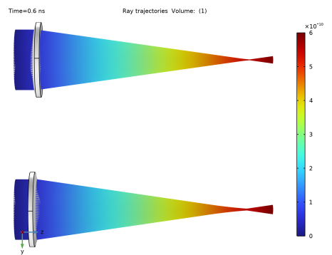
In the Model Builder window, expand the Results > Datasets node, then click Intersection Point 3D 1.
|
|
2
|
|
3
|
|
4
|
|
5
|
|
1
|
|
2
|
|
3
|
|
1
|
|
2
|
|
1
|
|
2
|
|
1
|
|
2
|
|
3
|
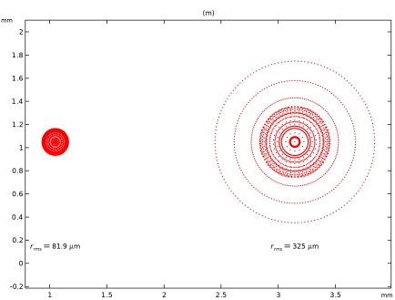
Select the Manual axis limits checkbox.
|
|
4
|
|
5
|
|
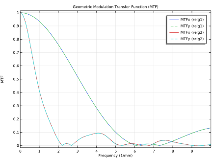
1
|
|
2
|
|
3
|
|
1
|
|
2
|
|
3
|