|
|
|
|
Ray direction vector, z-component
|
||
 |
Stop z-coordinate, where Tc,n is the central thickness of element n and Tn is the separation between elements n and n+1. Note that the stop is the third element in the Petzval lens.
|
|
 |
Image plane z-coordinate, where Tc,n is the central thickness of element n and Tn is the separation between elements n and n+1. Including the stop, the Petzval lens has 6 elements.
|
|
|
|
Athermal thickness of support i, where d is the lens diameter, αe, α1, and α2, are the CTEs of the elastomer, the mount, and the lens respectively, and νe is Poisson’s ratio.
|
|
•
|
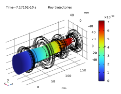
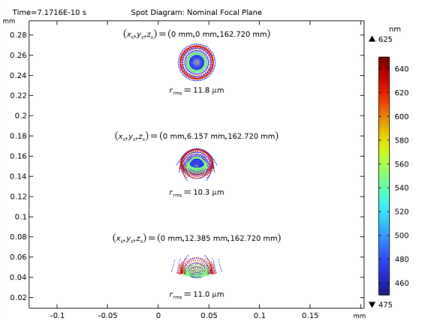
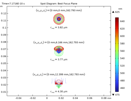
Petzval Lens STOP Analysis Isothermal Sweep — A parametric sweep over a range of uniform temperatures is performed. The position of the best focus image plane is determined as a function of temperature.
|
|
•
|
Petzval Lens STOP Analysis with Hyperelasticity — In this model the RTV lens supports are modeled as a hyperelastic material using the Nonlinear Structural Materials Module.
|
|
•
|
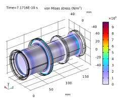
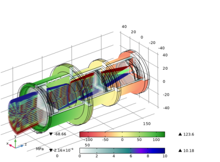
Petzval Lens STOP Analysis with Surface-to-Surface Radiation — For this model, the lens assembly is placed inside a thermo-vacuum enclosure where the exterior temperature is significantly different from the interior. The lens assembly is exposed to this exterior through a pair of windows via surface-to-surface radiation. The resulting thermal gradient and displacement field within the optical system are shown together with the effect on image quality.
|
|
1
|
|
2
|
|
3
|
Click Add.
|
|
4
|
|
5
|
Click Add.
|
|
6
|
Click
|
|
7
|
|
8
|
Click
|
|
1
|
|
2
|
In the Settings window for Geometry, type Petzval Lens Stop Analysis Geometry Sequence in the Label text field.
|
|
3
|
|
4
|
Browse to the model’s Application Libraries folder and double-click the file petzval_lens_stop_analysis_geom_sequence.mph.
|
|
5
|
|
6
|
|
7
|
|
8
|
|
9
|
|
10
|
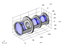
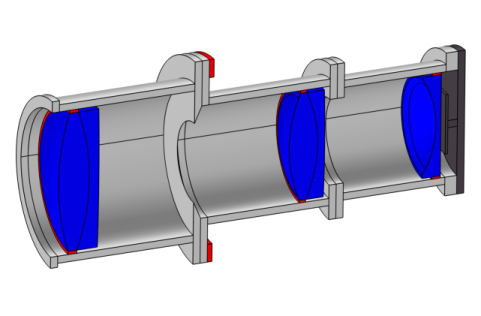
On the object fin, select Boundary 19 only. Continue to select boundaries that allow the inside of the lens assembly to be seen. Orient the view to match Figure 2.
|
|
1
|
|
2
|
In the Settings window for Parameters, type Lens Prescription in the Label text field. The lens prescription was added when the geometry sequence was inserted above. Next, create parameter nodes for material and general properties.
|
|
1
|
|
2
|
In the Settings window for Parameters, type Material Properties in the Label text field. These material properties contain other parameters than will be used in extensions of this study.
|
|
3
|
|
4
|
Browse to the model’s Application Libraries folder and double-click the file petzval_lens_stop_analysis_material_parameters.txt.
|
|
1
|
|
2
|
|
3
|
|
4
|
Browse to the model’s Application Libraries folder and double-click the file petzval_lens_stop_analysis_parameters.txt.
|
|
1
|
|
2
|
|
1
|
|
2
|
|
3
|
|
4
|
In the Add dialog, in the Selections to add list, choose All (Barrel 1), All (Barrel 2), All (Barrel 3), and Detector Assembly.
|
|
5
|
Click OK.
|
|
1
|
|
2
|
|
3
|
|
4
|
|
5
|
Click OK.
|
|
1
|
|
2
|
|
3
|
|
1
|
|
2
|
|
3
|
Click
|
|
1
|
|
2
|
|
3
|
Click
|
|
1
|
|
2
|
|
3
|
|
1
|
|
2
|
|
3
|
|
1
|
|
2
|
|
3
|
|
5
|
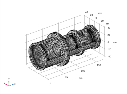
Locate the Element Size section. From the Predefined list, choose Finer. This is part of the detector assembly.
|
|
1
|
|
2
|
|
3
|
|
4
|
|
5
|
|
6
|
Locate the Element Size Parameters section.
|
|
7
|
|
1
|
|
2
|
|
3
|
|
1
|
|
2
|
|
3
|
|
4
|
Locate the Ray Release and Propagation section. From the Wavelength distribution of released rays list, choose Polychromatic, specify vacuum wavelength. The list of polychromatic wavelengths will be entered below.
|
|
5
|
In the Maximum number of secondary rays text field, type 0. In this simulation stray light is not being traced, so reflected rays will not be produced at the lens surfaces. Note that because rays will be traced through a deformed geometry, it is not possible to use geometry normals for ray-boundary interactions. This checkbox should remained cleared.
|
|
6
|
Locate the Material Properties of Exterior and Unmeshed Domains section. From the Optical dispersion model list, choose Air, Edlen (1953).
|
|
7
|
In the Text text field, type T0. The refractive index of the air surrounding the camera lens will be a function of temperature.
|
|
1
|
In the Model Builder window, under Component 1 (comp1) > Geometrical Optics (gop) click Medium Properties 1.
|
|
2
|
|
3
|
|
4
|
|
1
|
|
2
|
|
3
|
|
4
|
Find the Expression for remaining selection subsection. In the Temperature text field, type T0. This temperature is defined in the parameters node.
|
|
1
|
In the Model Builder window, under Component 1 (comp1) > Geometrical Optics (gop) click Material Discontinuity 1.
|
|
2
|
|
3
|
|
1
|
|
2
|
|
3
|
|
4
|
|
1
|
|
2
|
|
3
|
|
4
|
|
1
|
|
2
|
|
3
|
Locate the Boundary Selection section. From the Selection list, choose Image Plane. The default Wall condition is Freeze.
|
|
1
|
|
2
|
|
3
|
|
4
|
|
5
|
|
6
|
|
7
|
|
8
|
|
9
|
|
10
|
|
1
|
|
2
|
|
3
|
|
4
|
|
1
|
|
2
|
|
3
|
|
4
|
|
1
|
|
2
|
|
3
|
From the Displacement field list, choose Cubic serendipity. As for the Geometrical Optics interface, a cubic shape order is chosen to reduce discretization error.
|
|
1
|
|
1
|
|
2
|
|
3
|
From the Selection list, choose All (Rigid Support). It is assumed that the lens assembly is attached to an external rigid structure via this annulus. The external structure does not otherwise participate in the physics.
|
|
1
|
|
2
|
Go to the Add Material window.
|
|
3
|
|
4
|
Click the Add to Component button in the window toolbar.
|
|
5
|
|
6
|
Click the Add to Component button in the window toolbar.
|
|
7
|
|
8
|
Click the Add to Component button in the window toolbar.
|
|
9
|
|
10
|
Click the Add to Component button in the window toolbar.
|
|
11
|
|
1
|
|
2
|
|
1
|
|
2
|
|
3
|
|
1
|
|
2
|
|
3
|
|
1
|
|
2
|
|
3
|
|
1
|
|
2
|
Go to the Add Material window.
|
|
3
|
|
4
|
Click the Add to Component button in the window toolbar.
|
|
5
|
|
1
|
|
2
|
|
1
|
|
2
|
|
3
|
|
4
|
|
5
|
Locate the Material Contents section. In the table, enter the following settings:
|
|
1
|
|
2
|
|
3
|
|
4
|
|
5
|
In the Lengths text field, type 0 215. The maximum optical path length is sufficient to allow all rays to pass beyond the nominal location of the image plane.
|
|
6
|
Select the Include geometric nonlinearity checkbox. This ensures that the ray tracing is performed on the deformed geometry created in Step 1 of the Study.
|
|
7
|
Locate the Physics and Variables Selection section. In the Solve for column of the table, under Component 1 (comp1), clear the checkbox for Solid Mechanics (solid).
|
|
8
|
Select the Modify model configuration for study step checkbox.
|
|
9
|
|
10
|
Right-click and choose Disable.
|
|
11
|
|
1
|
|
2
|
|
3
|
|
4
|
From the Selection list, choose All Lenses. This selection is used to limit the domains in which some datasets will be processed.
|
|
1
|
|
2
|
|
3
|
|
4
|
|
5
|
|
6
|
|
7
|
|
8
|
|
9
|
|
10
|
|
11
|
|
12
|
|
1
|
|
2
|
|
3
|
|
4
|
|
5
|
|
6
|
Select the Show units checkbox.
|
|
7
|
|
8
|
|
9
|
|
1
|
|
2
|
|
3
|
|
1
|
|
2
|
|
3
|
In the Expression text field, type gop.prf. This is the Ray release feature index; that is, the field number.
|
|
4
|
|
5
|
|
1
|
|
2
|
|
3
|
|
4
|
In the Logical expression for inclusion text field, type at(0,qx>0.1[mm]). Restrict the rays visible to one half of the view. Also, rays are not rendered just beyond the nominal, undeformed image plane z-coordinate.
|
|
1
|
|
2
|
|
3
|
|
4
|
|
5
|
|
6
|
|
7
|
|
8
|
|
1
|
|
2
|
|
3
|
|
1
|
|
2
|
|
3
|
|
1
|
|
2
|
|
3
|
|
4
|
|
5
|
|
1
|
|
2
|
|
1
|
|
2
|
|
3
|
|
4
|
|
5
|
|
6
|
|
7
|
|
8
|
|
9
|
|
1
|
|
2
|
|
3
|
|
1
|
|
2
|
|
3
|
|
1
|
|
2
|
|
3
|
|
4
|
|
5
|
|
1
|
|
2
|
|
3
|
|
1
|
|
2
|
|
3
|
|
1
|
|
2
|
|
3
|
|
1
|
|
2
|
|
3
|
|
1
|
|
2
|
|
3
|
|
1
|
|
2
|
|
3
|
|
4
|
|
5
|
|
6
|
|
1
|
|
2
|
|
1
|
|
2
|
|
3
|
|
4
|
|
5
|
|
6
|
|
7
|
|
8
|
|
1
|
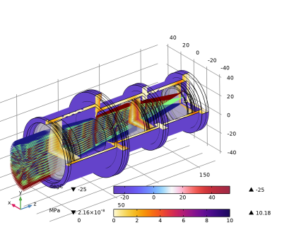
Right-click Surface 1 and choose Deformation. This is used to exaggerate the lens thermal deformation.
|
|
2
|
|
3
|
|
1
|
|
2
|
|
3
|
|
1
|
|
2
|
|
3
|
|
4
|
|
1
|
|
2
|
|
3
|
|
1
|
|
1
|
|
2
|
|
3
|
|
4
|
|
5
|
|
6
|
|
7
|
Select the Show units checkbox.
|
|
1
|
|
2
|
|
3
|
From the Image surface list, choose Intersection Point 3D 1. This is the Intersection Point 3D dataset defined above using three corners of the deformed image surface.
|
|
4
|
|
5
|
|
6
|
|
7
|
|
8
|
|
9
|
|
10
|
|
1
|
|
2
|
|
3
|
|
4
|
|
5
|
|
6
|
|
7
|
|
8
|
|
1
|
|
2
|
|
3
|
|
4
|
|
1
|
|
2
|
|
3
|
|
4
|
Locate the Filters section. Select the Filter by release feature index checkbox. The rays from the on-axis release will be used.
|
|
5
|
Click to expand the Focal Plane Orientation section. From the Normal to focal plane list, choose User defined. The default is that the image plane normal direction is the z-axis.
|
|
6
|
|
7
|
Click Create Focal Plane Dataset.
|
|
8
|
|
9
|
|
10
|
|
1
|
|
2
|
Click
|
|
1
|
|
2
|
|
3
|
|
4
|
|
5
|
|
6
|
Browse to the model’s Application Libraries folder and double-click the file petzval_lens_stop_analysis_petzval_lens_geom_sequence.mph. Following insertion, the full lens prescription will be available in the Parameters node.
|
|
1
|
|
2
|
|
3
|
Click
|
|
4
|
Browse to the model’s Application Libraries folder and double-click the file petzval_lens_stop_analysis_geom_sequence_parameters.txt.
|
|
1
|
|
2
|
|
3
|
In the Model Builder window, under Component 1 (comp1) click Petzval Lens STOP Analysis Geometry Sequence.
|
|
4
|
In the Settings window for Geometry, in the Graphics window toolbar, click
|
|
5
|
Click the
|
|
1
|
|
2
|
|
3
|
|
4
|
Locate the Input Parameters section. In the table, enter the following settings:
|
|
1
|
|
2
|
|
3
|
Locate the Input Parameters section. In the table, enter the following settings:
|
|
4
|
Locate the Position and Orientation of Output section. Find the Displacement subsection. In the zwi text field, type L1.
|
|
1
|
|
2
|
|
3
|
On the object pi1, select Boundary 1 only.
|
|
4
|
Locate the Distances section. In the table, enter the following settings:
|
|
1
|
|
2
|
|
3
|
Locate the Input Parameters section. In the table, enter the following settings:
|
|
1
|
|
2
|
|
3
|
On the object pi2, select Boundary 1 only.
|
|
4
|
Locate the Distances section. In the table, enter the following settings:
|
|
1
|
|
2
|
|
3
|
Locate the Input Parameters section. In the table, enter the following settings:
|
|
4
|
Locate the Position and Orientation of Output section. Find the Coordinate system to match subsection. From the Take work plane from list, choose Front Ring Annulus (pi2).
|
|
5
|
|
6
|
|
1
|
|
2
|
|
3
|
On the object pi3, select Boundary 1 only.
|
|
4
|
Locate the Distances section. In the table, enter the following settings:
|
|
5
|
Select the Reverse direction checkbox.
|
|
1
|
|
2
|
|
3
|
Click in the Graphics window and then press Ctrl+A to select all objects.
|
|
4
|
Locate the Selections of Resulting Entities section. Select the Resulting objects selection checkbox.
|
|
1
|
|
2
|
|
3
|
|
4
|
|
5
|
|
1
|
|
2
|
|
3
|
|
4
|
|
5
|
|
6
|
|
1
|
In the Model Builder window, under Component 1 (comp1) > Petzval Lens STOP Analysis Geometry Sequence click Group 1 Aperture (pi8).
|
|
2
|
|
1
|
|
2
|
|
1
|
|
2
|
|
4
|
Locate the Position and Orientation of Output section. Find the Displacement subsection. In the zwi text field, type 4.
|
|
1
|
|
2
|
|
3
|
On the object pi8, select Boundary 1 only.
|
|
4
|
|
5
|
On the object pi2, select Point 11 only.
|
|
6
|
Locate the Selections of Resulting Entities section. Find the Cumulative selection subsection. Click New.
|
|
7
|
|
8
|
Click OK.
|
|
1
|
|
2
|
|
3
|
On the object pi9, select Boundary 1 only.
|
|
4
|
|
5
|
On the object pi5, select Point 11 only.
|
|
6
|
Locate the Selections of Resulting Entities section. Find the Cumulative selection subsection. From the Contribute to list, choose Supports.
|
|
1
|
|
2
|
|
3
|
On the object pi10, select Boundary 1 only.
|
|
4
|
|
5
|
On the object pi6, select Point 12 only.
|
|
6
|
Locate the Selections of Resulting Entities section. Find the Cumulative selection subsection. From the Contribute to list, choose Supports.
|
|
7
|
|
1
|
|
2
|
|
3
|
Find the Coordinate system in part subsection. From the Work plane in part list, choose Front Plane (wp1).
|
|
4
|
Find the Coordinate system to match subsection. From the Take work plane from list, choose Lens 1 (pi1).
|
|
5
|
|
6
|
Locate the Input Parameters section. In the table, enter the following settings:
|
|
7
|
Locate the Position and Orientation of Output section. Find the Displacement subsection. In the zwi text field, type -3.0[mm].
|
|
8
|
|
1
|
|
2
|
|
3
|
|
4
|
|
5
|
|
6
|
|
7
|
|
8
|
|
1
|
|
2
|
Select the object pi11 only.
|
|
3
|
|
4
|
|
5
|
Select the object cone1 only.
|
|
1
|
|
2
|
|
3
|
Find the Coordinate system in part subsection. From the Work plane in part list, choose Front Plane (wp1).
|
|
4
|
Find the Coordinate system to match subsection. From the Take work plane from list, choose Barrel 1 (pi11).
|
|
5
|
|
6
|
Locate the Input Parameters section. In the table, enter the following settings:
|
|
7
|
|
1
|
|
2
|
|
3
|
Find the Coordinate system in part subsection. From the Work plane in part list, choose Front Plane (wp1).
|
|
4
|
Find the Coordinate system to match subsection. From the Take work plane from list, choose Barrel 2 (pi12).
|
|
5
|
|
6
|
Locate the Input Parameters section. In the table, enter the following settings:
|
|
7
|
|
1
|
|
2
|
|
3
|
|
1
|
|
2
|
|
3
|
|
4
|
|
5
|
|
6
|
|
7
|
|
1
|
|
2
|
|
3
|
|
4
|
|
5
|
|
6
|
|
1
|
|
2
|
|
3
|
|
4
|
Locate the Selections of Resulting Entities section. Select the Resulting objects selection checkbox.
|
|
1
|
|
2
|
|
3
|
Locate the Input Parameters section. In the table, enter the following settings:
|
|
4
|
Locate the Position and Orientation of Output section. Find the Coordinate system to match subsection. From the Take work plane from list, choose Barrel 2 (pi12).
|
|
5
|
|
6
|
|
7
|
|
1
|
|
2
|
|
3
|
On the object pi14, select Boundary 1 only.
|
|
4
|
Locate the Distances section. In the table, enter the following settings:
|
|
5
|
Select the Reverse direction checkbox.
|
|
6
|
Locate the Selections of Resulting Entities section. Find the Cumulative selection subsection. From the Contribute to list, choose Supports.
|
|
1
|
|
2
|
|
3
|
|
4
|
|
5
|
|
6
|
Click OK.
|
|
7
|