|
|
1
|
|
2
|
|
3
|
Click Add.
|
|
4
|
Click
|
|
5
|
|
6
|
Click
|
|
1
|
|
2
|
In the Settings window for Geometry, type Newtonian Telescope Structural Analysis Geometry Sequence in the Label text field.
|
|
3
|
|
4
|
|
5
|
Browse to the model’s Application Libraries folder and double-click the file newtonian_telescope_structural_analysis_geom_sequence.mph.
|
|
6
|
|
7
|
|
8
|
|
1
|
|
2
|
In the Settings window for Parameters, type Parameters 1: Telescope Geometry in the Label text field. The telescope geometry parameters were added when the geometry sequence was inserted.
|
|
3
|
Locate the Parameters section. In the table, enter the following settings:
|
|
1
|
|
2
|
In the Settings window for Parameters, type Parameters 2: Wavelengths and Fields in the Label text field.
|
|
3
|
|
4
|
Browse to the model’s Application Libraries folder and double-click the file newtonian_telescope_structural_analysis_parameters.txt.
|
|
2
|
|
3
|
|
4
|
Clear the Automatic detection of small details checkbox.
|
|
5
|
|
1
|
|
2
|
Go to the Add Material window.
|
|
3
|
|
4
|
Click the Add to Component button in the window toolbar.
|
|
5
|
|
6
|
Click the Add to Component button in the window toolbar.
|
|
7
|
|
8
|
Click the Add to Component button in the window toolbar.
|
|
9
|
|
1
|
|
1
|
|
2
|
|
3
|
Click
|
|
4
|
Locate the Ray Release and Propagation section. In the Maximum number of secondary rays text field, type 0.
|
|
5
|
Locate the Additional Variables section. Select the Compute optical path length checkbox. The optical path length will be used to create the aberration diagrams.
|
|
6
|
Select the Count reflections checkbox. The number of reflections (gop.Nrefl) can be used to control the behavior of physics features or during postprocessing.
|
|
1
|
In the Model Builder window, under Component 1 (comp1) > Geometrical Optics (gop) click Ray Properties 1.
|
|
2
|
|
3
|
|
1
|
|
2
|
|
3
|
|
4
|
|
5
|
|
6
|
|
7
|
|
8
|
|
1
|
|
2
|
|
3
|
|
4
|
|
5
|
|
1
|
|
2
|
|
3
|
Locate the Boundary Selection section. From the Selection list, choose Mirror surface (Primary Mirror).
|
|
1
|
|
2
|
|
3
|
Locate the Boundary Selection section. From the Selection list, choose Mirror surface (Secondary Mirror).
|
|
4
|
|
5
|
|
6
|
In the e text field, type gop.Nrefl>0. A ray striking the secondary mirror will reflect only if it has encountered a mirror surface (that is, the Primary Mirror) previously.
|
|
7
|
|
1
|
|
2
|
|
3
|
|
4
|
|
1
|
|
2
|
|
3
|
|
4
|
|
1
|
|
2
|
|
3
|
|
1
|
|
2
|
|
3
|
|
4
|
|
5
|
|
1
|
|
2
|
|
3
|
|
4
|
|
6
|
|
1
|
|
2
|
|
3
|
|
5
|
|
1
|
|
2
|
|
1
|
|
2
|
|
3
|
|
4
|
|
5
|
In the Lengths text field, type 0 2.10*f. The maximum path length is slightly greater than twice the focal length of the telescope. This ensures that all rays reach the focal plane.
|
|
6
|
|
1
|
|
2
|
|
3
|
|
1
|
In the Model Builder window, expand the Results > Ray Diagram - Undeformed > Ray Trajectories 1 node, then click Color Expression 1.
|
|
2
|
|
3
|
In the Expression text field, type at('last',gop.rrel). This colors the ray according to their radial distance of the centroid of each release feature on the image plane.
|
|
4
|
|
5
|
|
1
|
|
2
|
|
3
|
Locate the Plot Settings section.
|
|
4
|
|
5
|
|
6
|
|
1
|
|
2
|
|
3
|
From the Transverse direction list, choose User defined. This allows the orientation of the spot diagram to be controlled.
|
|
4
|
|
5
|
|
6
|
|
7
|
|
8
|
|
9
|
|
10
|
|
11
|
From the Coordinate system list, choose Global. Using the Global coordinate system allows the z coordinate to be displayed.
|
|
12
|
|
13
|
Select the Fit annotations to spot checkbox.
|
|
1
|
|
2
|
|
3
|
|
4
|
|
1
|
|
2
|
In the Settings window for 2D Plot Group, type Aberration Diagram - Undeformed in the Label text field.
|
|
3
|
|
1
|
|
2
|
|
3
|
Select the Filter by release feature index checkbox. By default, the first (on-axis) release is selected.
|
|
4
|
Locate the Focal Plane Orientation section. Click Create Reference Hemisphere Dataset. This will create an Intersection Point 3D dataset, with a reference hemisphere that is centered on the point that minimizes the on-axis RMS spot radius.
|
|
5
|
|
6
|
|
1
|
|
2
|
|
3
|
|
4
|
|
5
|
Locate the Zernike Polynomials section. From the Terms to include list, choose Select individual terms.
|
|
6
|
Select the Z(3,-1), vertical coma checkbox.
|
|
7
|
Select the Z(3,1), horizontal coma checkbox. As expected for a telescope with a parabolic primary mirror, the dominate off-axis aberration is coma.
|
|
8
|
|
9
|
|
1
|
|
2
|
Go to the Add Physics window.
|
|
3
|
In the tree, select Structural Mechanics > Solid Mechanics (solid). Next, ensure that the solid mechanics physics will not be considered in the existing study.
|
|
4
|
Find the Physics interfaces in study subsection. In the table, clear the Solve checkbox for Study 1.
|
|
5
|
Click the Add to Component 1 button in the window toolbar.
|
|
6
|
|
1
|
|
1
|
|
2
|
Go to the Add Study window.
|
|
3
|
Find the Studies subsection. In the Select Study tree, select Preset Studies for Some Physics Interfaces > Stationary.
|
|
4
|
Find the Physics interfaces in study subsection. In the table, clear the Solve checkbox for Geometrical Optics (gop).
|
|
5
|
Click the Add Study button in the window toolbar.
|
|
6
|
|
1
|
|
2
|
|
3
|
|
4
|
|
5
|
|
6
|
Select the Include geometric nonlinearity checkbox. Geometric nonlinearities must be included otherwise the ray trace will not be performed on the deformed telescope geometry.
|
|
7
|
Locate the Physics and Variables Selection section. In the Solve for column of the table, under Component 1 (comp1), clear the checkbox for Solid Mechanics (solid).
|
|
8
|
Select the Modify model configuration for study step checkbox.
|
|
9
|
|
10
|
Right-click and choose Disable.
|
|
11
|
|
1
|
|
2
|
|
3
|
|
1
|
In the Model Builder window, expand the Results > Ray Diagram - Deformed > Ray Trajectories 1 node, then click Color Expression 1.
|
|
2
|
|
3
|
Clear the Color legend checkbox.
|
|
1
|
|
2
|
|
3
|
|
4
|
|
5
|
|
6
|
|
1
|
|
2
|
|
1
|
|
2
|
|
1
|
|
2
|
Go to the Result Templates window.
|
|
3
|
|
4
|
Click the Add Result Template button in the window toolbar.
|
|
5
|
|
1
|
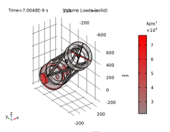
In the Model Builder window, expand the Applied Loads (solid) node, then click Volume Loads (solid).
|
|
2
|
|
1
|
|
2
|
|
3
|
Locate the Data section. From the Dataset list, choose Ray 2. This dataset was created when Study 2 was run. It is necessary to use this dataset when using the Automatic Focal Plane Calculation below.
|
|
1
|
|
2
|
|
3
|
Select the Filter by release feature index checkbox.
|
|
4
|
Locate the Focal Plane Orientation section. Click Create Focal Plane Dataset. This generates an Intersection Point 3D dataset that minimizes the RMS radius of the first ray release. The resulting point and normal values define the focal plane.
|
|
5
|
Locate the Filters section. Clear the Filter by release feature index checkbox. The intersection of all ray releases with the focal plane will now be shown.
|
|
6
|
|
1
|
|
2
|
In the Settings window for 2D Plot Group, type Aberration Diagram - Deformed in the Label text field.
|
|
3
|
|
4
|
|
1
|
|
2
|
|
3
|
Select the Filter by release feature index checkbox.
|
|
4
|
Locate the Focal Plane Orientation section. Click Create Reference Hemisphere Dataset. Similar to the spot diagram, this generates an Intersection Point 3D dataset that is centered on the plane that minimizes the RMS radius of the first ray release. The reference hemisphere center and axis direction should be identical to the point and normal values in Intersection Point 3D 1 which also define the focal plane.
|
|
5
|
Locate the Zernike Polynomials section. From the Terms to include list, choose Select individual terms.
|
|
6
|
Select the Z(2,0), defocus checkbox.
|
|
7
|
Select the Z(3,-1), vertical coma checkbox.
|
|
8
|
Select the Z(3,1), horizontal coma checkbox. In this diagram, the defocus term now dominates.
|
|
9
|
|
10
|
|
1
|
|
2
|
|
3
|
|
4
|
|
5
|
|
6
|
|
1
|
|
2
|
|
3
|
Click Add.
|
|
4
|
Click
|
|
5
|
|
6
|
Click
|
|
1
|
|
2
|
In the Settings window for Geometry, type Newtonian Telescope Structural Analysis Geometry Sequence in the Label text field.
|
|
3
|
|
4
|
|
5
|
Browse to the model’s Application Libraries folder and double-click the file newtonian_telescope_structural_analysis_geom_sequence.mph.
|
|
6
|
|
7
|
|
8
|
|
1
|
|
2
|
In the Settings window for Parameters, type Parameters 1: Telescope Geometry in the Label text field. The telescope geometry parameters were added when the geometry sequence was inserted.
|
|
3
|
Locate the Parameters section. In the table, enter the following settings:
|
|
1
|
|
2
|
In the Settings window for Parameters, type Parameters 2: Wavelengths and Fields in the Label text field.
|
|
3
|
|
4
|
Browse to the model’s Application Libraries folder and double-click the file newtonian_telescope_structural_analysis_parameters.txt.
|
|
2
|
|
3
|
|
4
|
Clear the Automatic detection of small details checkbox.
|
|
5
|
|
1
|
|
2
|
Go to the Add Material window.
|
|
3
|
|
4
|
Click the Add to Component button in the window toolbar.
|
|
5
|
|
6
|
Click the Add to Component button in the window toolbar.
|
|
7
|
|
8
|
Click the Add to Component button in the window toolbar.
|
|
9
|
|
1
|
|
1
|
|
2
|
|
3
|
Click
|
|
4
|
Locate the Ray Release and Propagation section. In the Maximum number of secondary rays text field, type 0.
|
|
5
|
Locate the Additional Variables section. Select the Compute optical path length checkbox. The optical path length will be used to create the aberration diagrams.
|
|
6
|
Select the Count reflections checkbox. The number of reflections (gop.Nrefl) can be used to control the behavior of physics features or during postprocessing.
|
|
1
|
In the Model Builder window, under Component 1 (comp1) > Geometrical Optics (gop) click Ray Properties 1.
|
|
2
|
|
3
|
|
1
|
|
2
|
|
3
|
|
4
|
|
5
|
|
6
|
|
7
|
|
8
|
|
1
|
|
2
|
|
3
|
|
4
|
|
5
|
|
1
|
|
2
|
|
3
|
Locate the Boundary Selection section. From the Selection list, choose Mirror surface (Primary Mirror).
|
|
1
|
|
2
|
|
3
|
Locate the Boundary Selection section. From the Selection list, choose Mirror surface (Secondary Mirror).
|
|
4
|
|
5
|
|
6
|
In the e text field, type gop.Nrefl>0. A ray striking the secondary mirror will reflect only if it has encountered a mirror surface (that is, the Primary Mirror) previously.
|
|
7
|
|
1
|
|
2
|
|
3
|
|
4
|
|
1
|
|
2
|
|
3
|
|
4
|
|
1
|
|
2
|
|
3
|
|
1
|
|
2
|
|
3
|
|
4
|
|
5
|
|
1
|
|
2
|
|
3
|
|
4
|
|
6
|
|
1
|
|
2
|
|
3
|
|
5
|
|
1
|
|
2
|
|
1
|
|
2
|
|
3
|
|
4
|
|
5
|
In the Lengths text field, type 0 2.10*f. The maximum path length is slightly greater than twice the focal length of the telescope. This ensures that all rays reach the focal plane.
|
|
6
|
|
1
|
|
2
|
|
3
|
|
1
|
In the Model Builder window, expand the Results > Ray Diagram - Undeformed > Ray Trajectories 1 node, then click Color Expression 1.
|
|
2
|
|
3
|
In the Expression text field, type at('last',gop.rrel). This colors the ray according to their radial distance of the centroid of each release feature on the image plane.
|
|
4
|
|
5
|
|
1
|
|
2
|
|
3
|
Locate the Plot Settings section.
|
|
4
|
|
5
|
|
6
|
|
1
|
|
2
|
|
3
|
From the Transverse direction list, choose User defined. This allows the orientation of the spot diagram to be controlled.
|
|
4
|
|
5
|
|
6
|
|
7
|
|
8
|
|
9
|
|
10
|
|
11
|
From the Coordinate system list, choose Global. Using the Global coordinate system allows the z coordinate to be displayed.
|
|
12
|
|
13
|
Select the Fit annotations to spot checkbox.
|
|
1
|
|
2
|
|
3
|
|
4
|
|
1
|
|
2
|
In the Settings window for 2D Plot Group, type Aberration Diagram - Undeformed in the Label text field.
|
|
3
|
|
1
|
|
2
|
|
3
|
Select the Filter by release feature index checkbox. By default, the first (on-axis) release is selected.
|
|
4
|
Locate the Focal Plane Orientation section. Click Create Reference Hemisphere Dataset. This will create an Intersection Point 3D dataset, with a reference hemisphere that is centered on the point that minimizes the on-axis RMS spot radius.
|
|
5
|
|
6
|
|
1
|
|
2
|
|
3
|
|
4
|
|
5
|
Locate the Zernike Polynomials section. From the Terms to include list, choose Select individual terms.
|
|
6
|
Select the Z(3,-1), vertical coma checkbox.
|
|
7
|
Select the Z(3,1), horizontal coma checkbox. As expected for a telescope with a parabolic primary mirror, the dominate off-axis aberration is coma.
|
|
8
|
|
9
|
|
1
|
|
2
|
Go to the Add Physics window.
|
|
3
|
In the tree, select Structural Mechanics > Solid Mechanics (solid). Next, ensure that the solid mechanics physics will not be considered in the existing study.
|
|
4
|
Find the Physics interfaces in study subsection. In the table, clear the Solve checkbox for Study 1.
|
|
5
|
Click the Add to Component 1 button in the window toolbar.
|
|
6
|
|
1
|
|
1
|
|
2
|
Go to the Add Study window.
|
|
3
|
Find the Studies subsection. In the Select Study tree, select Preset Studies for Some Physics Interfaces > Stationary.
|
|
4
|
Find the Physics interfaces in study subsection. In the table, clear the Solve checkbox for Geometrical Optics (gop).
|
|
5
|
Click the Add Study button in the window toolbar.
|
|
6
|
|
1
|
|
2
|
|
3
|
|
4
|
|
5
|
|
6
|
Select the Include geometric nonlinearity checkbox. Geometric nonlinearities must be included otherwise the ray trace will not be performed on the deformed telescope geometry.
|
|
7
|
Locate the Physics and Variables Selection section. In the Solve for column of the table, under Component 1 (comp1), clear the checkbox for Solid Mechanics (solid).
|
|
8
|
Select the Modify model configuration for study step checkbox.
|
|
9
|
|
10
|
Right-click and choose Disable.
|
|
11
|
|
1
|
|
2
|
|
3
|
|
1
|
In the Model Builder window, expand the Results > Ray Diagram - Deformed > Ray Trajectories 1 node, then click Color Expression 1.
|
|
2
|
|
3
|
Clear the Color legend checkbox.
|
|
1
|
|
2
|
|
3
|
|
4
|
|
5
|
|
6
|
|
1
|
|
2
|
|
1
|
|
2
|
|
1
|
|
2
|
Go to the Result Templates window.
|
|
3
|
|
4
|
Click the Add Result Template button in the window toolbar.
|
|
5
|
|
1
|
In the Model Builder window, expand the Applied Loads (solid) node, then click Volume Loads (solid).
|
|
2
|
|
1
|
|
2
|
|
3
|
Locate the Data section. From the Dataset list, choose Ray 2. This dataset was created when Study 2 was run. It is necessary to use this dataset when using the Automatic Focal Plane Calculation below.
|
|
1
|
|
2
|
|
3
|
Select the Filter by release feature index checkbox.
|
|
4
|
Locate the Focal Plane Orientation section. Click Create Focal Plane Dataset. This generates an Intersection Point 3D dataset that minimizes the RMS radius of the first ray release. The resulting point and normal values define the focal plane.
|
|
5
|
Locate the Filters section. Clear the Filter by release feature index checkbox. The intersection of all ray releases with the focal plane will now be shown.
|
|
6
|
|
1
|
|
2
|
In the Settings window for 2D Plot Group, type Aberration Diagram - Deformed in the Label text field.
|
|
3
|
|
4
|
|
1
|
|
2
|
|
3
|
Select the Filter by release feature index checkbox.
|
|
4
|
Locate the Focal Plane Orientation section. Click Create Reference Hemisphere Dataset. Similar to the spot diagram, this generates an Intersection Point 3D dataset that is centered on the plane that minimizes the RMS radius of the first ray release. The reference hemisphere center and axis direction should be identical to the point and normal values in Intersection Point 3D 1 which also define the focal plane.
|
|
5
|
Locate the Zernike Polynomials section. From the Terms to include list, choose Select individual terms.
|
|
6
|
Select the Z(2,0), defocus checkbox.
|
|
7
|
Select the Z(3,-1), vertical coma checkbox.
|
|
8
|
Select the Z(3,1), horizontal coma checkbox. In this diagram, the defocus term now dominates.
|
|
9
|
|
10
|
|
1
|
|
2
|
|
3
|
|
4
|
|
5
|
|
6
|